Formalizing Moessner's Theorem in Nuprl

By: Mark Bickford, Dexter Kozen & Alexandra Silva

May 23, 2012

Abstract

Moessner's theorem describes a procedure for generating a sequence of n integer sequences that lead unexpectedly to the sequence of nth powers 1ⁿ, 2ⁿ, 3ⁿ, … . Several generalizations of Moessner's theorem exist. Recently, Kozen and Silva gave an algebraic proof of a general theorem that subsumes Moessner's original theorem and its know generalizations. In this note, we describe the formalization of this theorem that the first author did in Nuprl. To the best of our knowledge, this is the first existing machine formalization. On the one hand, the formalization remains remarkably close to the original proof. On the other hand, it lead to new insights in the proof, pointing to small gaps and ambiguities that would never raise any objections in pen and pencil proofs, but which must be resolved in machine formalization.

Introduction

Proof assistants or interactive theorem provers are software tools used for formalizing properties and proofs of those properties. The holy grail of mechanized theorem proving is to give formalized, machine-checked mathematical proofs that are as close to the human written proofs as possible.

The Nuprl ("new pearl") proof development system is based on a formal account of deduction. Proofs are the main characters and are used not only to establish truth but also to denote evidence, including computational evidence in the form of programs (functional and distributed). The idea of a proof term is a key abstraction; it is a meaningful mathematical expression denoting evidence for truth.

In this note, we describe the formalization in Nuprl of the recent proof of Kozen and Silva  [5] of Moessner's theorem and its generalizations. The process of formalization uncovered several idiosyncrasies that forced us to be much more precise in several points than we had been in the paper proof. The main challenge was to build all the needed mathematical background. Once this was in place, the formal statements and their proofs turned out to be relatively straightforward and close to the originals.

We will omit most of the details of the proofs, referring the reader to  [5] for further details. Instead, we will walk the reader through the steps that had to be taken to obtain a full formalization and we will point out the unexpected differences with the proof in  [5] and the challenges faced during the formalization. But first, let us describe the problem we will formalize.

Consider the following procedure for generating n ≥ 1 infinite sequences of positive integers. To generate the first sequence, write down the positive integers 1, 2, 3, …, then cross out every nth element. For the second sequence, compute the prefix sums of the first sequence, ignoring the crossed-out elements, then cross out every (n- 1)st element. For the third sequence, compute the prefix sums of the second sequence, then cross out every (n- 2)nd element, and so on. For example, for n = 4,

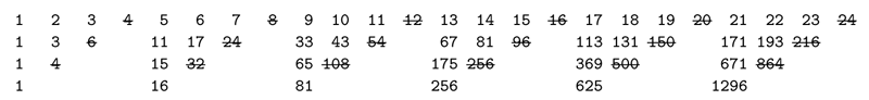
Moessner's theorem says that the final sequence is 1ⁿ,  2ⁿ,  3ⁿ,  … .

This construction is an interesting combinatorial curiosity that has attracted much attention over the years. The theorem was never proved by its eponymous discoverer  [8]. The first proof was given by Perron  [13]. The theorem has been the subject of several popular accounts  [1, 3, 7].

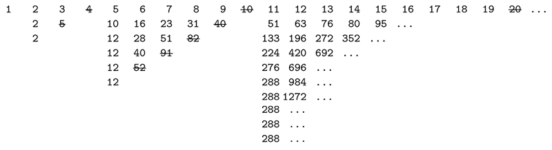
In the construction of Moessner's theorem, the initial step size n is constant. What happens if we increase it in each step? Let us repeat the construction starting with a step size of one and increasing the step size by one each time. Thus, in the first sequence, we cross out 1, 3, 6, 10, …, , … .

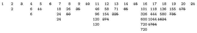
Let us now increment the increment by one in each step, thus incrementing the step size by 1, 2, 3, 4, … in successive steps, crossing out 1, 4, 10, 20, …, , … .

The final sequence consists of the superfactorials

1, 2, 12, 288, …

= 1!, 2!1!, 3!2!1!, 4!3!2!1!, … = 1!!, 2!!, 3!!, 4!!, … .

The generalization of Moessner's theorem that handles these cases is known as Paasche's theorem  [10, 11, 12].

Long  [6, 7] discovered the following alternative procedure and generalization. Consider the figure illustrating the Moessner construction for n = 4 above. Breaking the figure into separate triangles and adding a row of 1's at the top, the first four triangles are

Call these the level-nMoessner triangles. The first triangle is the Pascal triangle. However, note that all the triangles satisfy the Pascal property: each interior element is the sum of the elements immediately above it and to its left.

Instead of a sequence of sequences of integers, Long described how to generate a single sequence of triangles. To generate the (k + 1)st triangle from the kth, consider the nth northeast-to-southwest row. (For the second triangle above, this would be 1 8 24 32 16.) Let the first column of the next triangle be the prefix sums of this sequence (in our example, 1 9 33 65 81), and let the first row be a sequence of 1's. Complete the triangle using the Pascal property.

Long  [6, 7] and Salié  [14] also generalized Moessner's result to apply to the situation in which the first sequence is not the sequence of successive integers 1, 2, 3, … but the arithmetic progression a, a + d, a + 2d, … . This corresponds to a sequence of triangles with d, d, d, … along the top and d, a, a, a, … as the first column of the first triangle. They showed that the final sequence obtained by the Moessner construction is a⋅ 1^n-1, (a + d) ⋅ 2^n-1, (a + 2d) ⋅ 3^n-1, … .

Very recently, Hinze  [2] and Niqui and Rutten  [9] have given proofs involving concepts from functional programming, Hinze using calculational scans and Niqui and Rutten using coalgebra of streams. The proof of Hinze covers Moessner's and Paasche's result whereas Rutten and Niqui only provide a proof of the original Moessner's theorem.

The proof Kozen and Silva presented in  [5] has the advantage of covering all the theorems mentioned above and, furthermore, opening the door to new generalizations of Moessner's original result.

Algebraic Representation: Formal Power Series

Kozen and Silva described Long's construction in terms of multidimensional generating functions, also known as formal power series in multiple variables.

The first step taken was to formalize the theory of formal power series. In Nuprl, there were already formalizations of basic algebraic structures, such as monoids, groups and rings (described in Paul Jackson's thesis  [4]) and also of multisets (or bags). This made it possibly to incrementally build the theory of formal power series: a formal power series is represented as a map between monomials and coefficients taken from a ring. A monomial, in turn, is just a multiset of variables. The operations on formal power series, such as sum and convolution product, were then simply defined reusing existing operations on multisets. The details of this formalization are not important to understand the rest of the paper and will therefore be omitted.

The triangles were represented as elements of the rational function field Z(x, y). For example, the Pascal triangle Δ = Δ(x, y) is

Δ(x, y) = .

(1)

In Nuprl, this is represented concisely by the statement:

Δ (x,y) == (1 ÷ (1-(<{x}>+<{y}>)))

Note the close similarity to the formula (1) above.

A power series in x, y is called Pascal if the coefficient of every interior monomial m (a monomial of positive degree in both x and y) is the sum of the coefficients of m/x and m/y. The following lemma from  [5] characterizes the Pascal property of a power series:

In Nuprl the formal statement of this lemma is very close to the original formulation:

Here we see how the formalization forces us to be more precise: when one writes x and y for the variable names, one is implicitly assuming that they are different. However, in the formalization this needs to be said explicitly. The same applies to quantification: in the formulation of Lemma 2.1 above, the symbol f refers to any formal power series, which is made precise in the ∀ quantification of the Nuprl code. Furthermore, note that we need not restrict ourselves to the ring of integers as in the original proof, but instead can generalize to any commutative ring, which we denote by r:CRng.

Before describing how the successive triangles are constructed, one more result is needed: that any two given series g ∈Z(x) and f ∈Z(y) with the same constant coefficient can be extended uniquely to a p ∈Z(x, y) satisfying the Pascal property.

To formalize this, we first define the equation (2) as

In the original proof, a parameter p₀ was used in place of f(0) = g(0) so that the statement of the theorem would be symmetric in g and f. Here we have used f(0) (in Nuprl, f(y:=0)) instead. This breaks the symmetry but avoids having to define the extra parameter p₀.

Next, to finish the formalization of Lemma 2.2, we need to state and prove the uniqueness of p, which we are here denoting by Pascal-completion(r;f;g;x;y):

The first three conjuncts correspond to (i), (ii) and (iii) in Lemma 2.2 and the last conjunct to the statement of uniqueness.

Some remarks are in order for the code after the supposing clause. First, in the formalization above, we have not actually restricted f and g to be power series in one variable. Instead, we take any series in any number of variables, then require that f and g satisfy (f(x:=0) = f) ∧ (g(y:=0) = g), which is enough for the proof. This is a generalization of the original Lemma 2.2 above. Moreover, in the process of doing the proof, we discovered that the statement does not hold for the trivial ring, thus we need the additional assumption (¬(1 = 0)). The original proof was done in the ring of integers, in which this statement holds trivially.

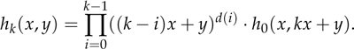
Each successive level-n Moessner triangle is obtained from the previous by taking the homogeneous component of degree n, evaluating at y = 1, and multiplying by Δ. In other words, if we define inductively

h0(x, y)= 1

hk+1(x, y) = n,

(3)

then the kth level-n Moessner triangle is h_k(x, 1) ⋅ Δ and the final sequence in the Moessner construction is the lead coefficient of h_k(x, 1) for k = 1, 2, 3, … .

We first need to define the operation of taking the homogeneous component of degree n. Because of the formalization of power series using bags of monomials, this is a rather simple operation:

Next, we formalize the operation of evaluating at y = 1:

We are now ready to state and formalize the main lemma of the paper.

In Nuprl, this was formalized as:

∀[r:CRng]. ∀[x,y:Atom]. ∀[h:PowerSeries(r)]. ∀[n,m:]. [([h]_n(y:=1)*Δ(x,y))]_m = ([h]_n(y:=(x+y))*((x+y))^(m - n)) supposing (n ≤ m) ∧ (¬ (x = y))

The main difference between this formalization and Lemma 2.3 is that we do not assume h(x, y) to be homogeneous of degree n, but instead take its homogeneous component of degree n: [h]_n. Variable m in the formalization above corresponds to n + d in Lemma 2.3.

Next, we present the main theorem of the paper, which has as corollaries Moessner's theorem and the several generalizations mentioned in the introduction.

Theorem 2.4 ( [5]) Let h_k be the sequence defined by (3). For all k ≥ 0,

The formalization in Nuprl is:

∀[r:CRng]. ∀[x,y:Atom]. ∀[h:PowerSeries(r)]. ∀[d:→ ]. ∀[k:].
Moessner(r;x;y;h;d;k) = ([h]_d0(y:=((k ⋅ r 1)*x + y)) * Π(i∈upto(k)).((((k - i) ⋅ r 1)*x + y))^(d (i + 1))) supposing ¬ (x = y)

Paasche's, Long's, and Moessner's theorems are now immediate consequences of Theorem 2.4.

Corollary 2.7 (Paasche's Theorem) For h₀ = 1 and any sequence d, the lead coefficient of h_k(x, 1) is

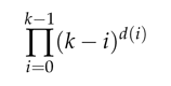
for all k ≥ 0. In particular, the sequences d = 1, 1, 1, …and d = 1, 2, 3, …yield the factorials and superfactorials, respectively.

References