
The Book
Implementing Mathematics with The Nuprl Proof Development System
See title page for important information about this reference
Next: Bibliography Up: doc Previous: Mathematics Libraries Contents
- Inductive Types
- Details of the Extension
- Example Proof
- Partial Function Types
- Details of the Extension
- General Notes
- Refinement Functions
- Rule Constructors
- Rule Destructors
- Term Destructors
- Auto-Tactic
- Miscellaneous Functions
- Differences in the Logic
- Differences in the User Interfaces
- Simulating Lambda-prl Constructs in Nuprl
Recursive Definition
For anyone doing mathematics or programming, recursive definition needs no motivation; its expressiveness, elegance and computational efficiency motivate us to include forms of it in the Nuprl logic. Current work on extending the logic involves three type constructors: rec, the inductive type constructor, permitting inductive data types and predicates; inf, the lazy type constructor, permitting infinite objects; and
Inductive Types
As an introduction to the rec types, consider the inductive type of integer trees, defined informally asIn the language of rec types this type may be defined as
rec(z. int | z#z).
Its elements include
inl 2,An inductive type may also be parameterized; generalizing the above definition of binary integer trees to general binary trees over a specified type, the example rephrased as
inr <inl 3,inl 5> and
inr <inr <inl 7,inl 11>,inl 13>.
is denoted
rec(z,x. x | z(x)#z(x); int),
and the predicate function dom,
asserting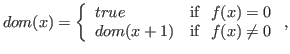
\x. rec(dom,x. int_eq(f(x); 0; true; dom(x+1)); x).
The elim form, rec_ind, is analogous to the list_ind and integer
ind forms. If t is of type rec(z. int | z#z) then
the following term computes the sum of the values at t's leaves.
     rec_ind(t;  sum,x.
       decide(x;
         leaf. leaf;
         pair. spread(pair; left_son,right_son.
                 sum(left_son)+sum(right_son))))
The simpler rec(
Expressiveness and Elegance
The transfinite W-type of well-founded trees,
     d:N#ind(d; x,y.void; void; x,T. Atomic_Stmt | (T#T) |
                                     (expr#T) | expr#T#T),
can be written more elegantly as
rec(T. Atomic_Stmt | (T#T) | (expr#T) | expr#T#T).
The list type constructor is now redundant because
Details of the Extension
The following modifications will add inductive types to Nuprl.
Computation System Modification
Add termsrec(where,
.
;
)
rec_ind(;
,
.
)
No instance ofThus (A#
rec_ind terms are noncanonical. These noncanonical terms
are redices with principal argument when\.rec_ind(,
- In rec(,.;)the and in front of the dot and
any free occurrences of or in become bound.
- In
rec_ind(; ,.)
the and in front of the dot and
any free occurrences of or in become bound.
Inductive Type Proof Rules
The proof rules will ensure that the following two assertions hold.rec(.
;
) type

&
->U
)->
That is, rec(rec(
&\![$,\;b/x,\;y]$](img840.png)
Formation
A universe intro rule such as ``»by intro rec'' cannot be phrased easily in the refinement logic style because of the syntactic restriction on
1.,
ggggggby ind
foobar][
»
Intro
2.![$[EXT r]$](img842.png)
»\![$,\;a/z,\;x]$](img844.png)
» rec(
3.
»\
» rec(
4._ind(;
,
.
![$G[p/p_2]$](img846.png)
by introover
using
![$Z[,p_2]$](img848.png)
:(
(
,
)»
![$G[p_1/p_2]$](img852.png)
»
Elim
5.»
![$[EXT t]$](img854.png)
\
6.rec
_ind(<)
by elimnew
![$h,Z[,p]$](img858.png)
![$[EXT g]$](img859.png)
»
Computation
7._ind(.
in
»\_ind(=
Example Proof
The
     ~<T>== (<T>) -> void
     some <v>:<A>.<P>== <v>:(<A>)#(<P>)
     N== {n:int| ~(n<0)}
     true== (0 in int)
     D(<x>)== rec(dom,x. int_eq(f(x); 0; true; dom(x+1)); <x>)
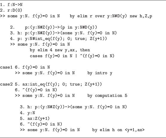
figure 12.1 sketches the proof of
f:N->N, r:D(0) >> some y:N. f(y)=0.
Although D(0) is inhabited only by axiom,
evaluating the extracted term produces a root.
Partial Function Types
We handle partial functions by viewing them as total functions over their domains of convergence. To do so we introduce dom terms, which capture the notion of a domain of convergence. Thus, for a partial function application to be sensible one must prove that the domain of convergence predicate is true for the argument, i.e., that the argument is in the domain of convergence of the function. The introduction of dom terms introduces additional proof obligations into the rules for reasoning about partial functions.
As an example,
the partial function ![]() producing the smallest root
producing the smallest root ![]() of
of ![]() ,
,
has a domain of convergence defined by the predicate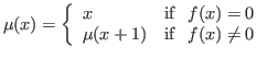
Thus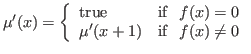
In our notation the type of partial
functions from ![]() to
to ![]() is
is
![]()
![]()
![]() , the application of partial function
, the application of partial function f to a is
written f[a], recursive functions are expressed as
terms of the form fix(![]() ,
,![]() .
.![]() ), so
function
), so
function ![]() of the preceding example is
of the preceding example is
MU == fix(mu,x. int_eq(f(x); 0; x; mu[x+1])),
and dom(MU) , an elim form
which turns out to have value
\x.rec(mu',x. int_eq(f(x); 0; true; mu(x+1)); MU; x).
The domain predicate is derived later;
in general,
if \[]
{}->As a second example, the ``91'' function,
has domain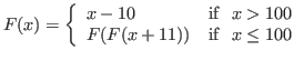
In our notation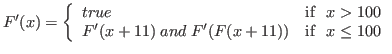
     91== fix(F,x. less(100; x; x-10; F[F[x+11]])

     \x.rec(F',x.
        less(100; x; true; c:F'(x+11)#F'(F[x+11]); 91; x)
Notice that the rec forms defined in the preceding section
must be extended to include the simultaneous definition of the
recursive function.
The new proof rules for these rec terms are only slight
variants of the given rules, so they are not listed here.
Details of the Extension
Computation System Modification
The domain predicate captures a call-by-value order of computation, so the entire computation system must be adjusted slightly to reflect this. In particular, computing the value of a function application (total or partial) dictates that function and argument are normalized before beta reduction, both subterms in pairs are normalized, and for injections into disjoint sums the subterm is normalized. In this extension direct computation rules are not present.
To add ![]() types to the logic we add terms
types to the logic we add terms
fix(where,
dom([]
Let ![]() stand for fix(
stand for fix(![]() ,
,![]() .
.![]() ) henceforth.
Each closed term
) henceforth.
Each closed term ![]() [
[![]() ] is a redex with contractum
] is a redex with contractum
![]() ,
and each closed term
dom(
,
and each closed term
dom(![]() ) is a redex with contractum
) is a redex with contractum
where\,
b
;
;
- In fix(,.), the and in front of the dot and
any free occurrences of or in become bound.
Domain Predicate
We define-
[] =
#'(),
if
had been bound by the the first variable in a surrounding fix term.
Recall that is the characteristic function for the domain of .
-
[] =
#
#dom()() if the first clause does not apply.
-
() =
#
-
spread(
 ; ,.) =
#spread(; ,.
), and
similarly for the other elimination forms.
; ,.) =
#spread(; ,.
), and
similarly for the other elimination forms.
-
inl() =
-
<,> =
#
-
=
true, for the remaining terms.
Partial Function Type Proof Rules
In the following
Formation
8.
»
»
Intro
9.
»
10.in
»
»
»{}={}in
{}»
11.
»
»{}
12.
»
»
Elim
13.
{}
Computation
14.
»=
General Notes
All universe levels must be strictly positive. Unless otherwise stated the tokens `nil` and `NIL` may be used as identifiers to indicate that no identifier should label the new hypothesis.
Refinement Functions
- refine: rule
 tactic.
 - This function refines a proof according to a given rule.
- refine_using_prl_rule: tok tactic.
- This function parses the token as a rule in the context of the
given proof. The proof is then refined via this rule.
Rule Constructors
See chapter 8 for a description of the rule constructors.
Rule Destructors
- rule_kind: rule tok.
- Returns the kind of the rule. Note that at present this is in
the internal form of the rule name. There are also predicates
of the form is_universe_intro_void that correctly
translate from the internal names of rules and the names of the rule
constructors (as listed above with ``is_'' prepended).
There are also destructors for each of the rules that correspond
to the constructor. The names are of the form
``destruct_universe_intro_void''.
Term Destructors
- term_kind: term -> tok.
- Returns the kind of the term. Possible results are: UNIVERSE,
VOID, ANY, ATOM, TOKEN, INT, NATURAL-NUMBER, MINUS, ADDITION, SUBTRACTION,
MULTIPLICATION, DIVISION, MODULO,
INTEGER-INDUCTION, LIST, NIL, CONS,
LIST-INDUCTION, UNION, INL, INR, DECIDE, PRODUCT, PAIR, SPREAD, FUNCTION, LAMBDA, APPLY, QUOTIENT, SET, EQUAL, AXIOM, VAR, BOUND-ID, TERM-OF-THEOREM, ATOMEQ, INTEQ, INTLESS.
There are corresponding predicates such as is_universe_term and corresponding constructors such as make_function_term (which has type tok
term term term).
- destruct_universe: term int.
- The integer is the universe
level.
- destruct_any: term term.
- destruct_token: term tok.
- destruct_natural_number: term int.
- destruct_minus: term term.
- destruct_addition: term (term # term).
-
The results are the left and right terms. - destruct_subtraction: term (term # term).
- destruct_multiplication: term (term # term).
- destruct_division: term (term # term).
- destruct_modulo: term (term # term).
- destruct_integer_induction: term (term # term # term # term).
-
The results are the value, down term, base term and up term. - destruct_list: term term.
- Returns the type of the list.
- destruct_cons: term (term # term).
- Returns the head and
tail.
- destruct_list_induction: term (term # term # term).
-
Returns the value, base term and up term. - destruct_union: term (term # term).
-
Results in the left and right types. - destruct_inl: term term.
- destruct_inr: term term.
- destruct_decide: term (term # term # term).
-
The result is the value, the left term and the right term. - destruct_product: term (tok # term # term).
-
The result is the bound identifier, the left term and the right term. - destruct_pair: term (term # term).
-
Returns the left term and the right term. - destruct_spread: term (term # term).
-
Returns the value and the term. - destruct_function: term (tok # (term # term)).
-
The result is the bound identifier, the left term and the right term. - destruct_lambda: term (tok # term).
-
Returns the bound identifier and the term. - destruct_apply: term (term # term).
-
Returns the function and the argument. - destruct_quotient: term (tok # (tok # (term # term))).
-
Returns the two bound identifiers, the left type and the right type. - destruct_set: term (tok # (term # term)).
-
Returns the bound identifier, the left type and the right type. - destruct_var: term tok.
- destruct_equal: term ((term list) # term).
-
Returns a list of the equal terms and the type of the equality. - destruct_less: term (term # term)).
-
Returns the left term and the right term. - destruct_bound_id: term ((tok list) # term).
-
Returns a list of the bound identifiers and the type. - destruct_term_of_theorem: term tok.
-
Returns the name of the theorem. - destruct_atomeq: term (term # (term # (term # term))).
-
Returns the left term, right term, if term and else term. - destruct_inteq: term (term # (term # (term # term))).
-
Returns the left term, right term, if term and else term. - destruct_intless: term (term # (term # (term # term))).
-
Returns the left term, right term, if term and else term. - destruct_tagged: term (int # term).
-
The integer returned is zero if the tag is *.
For each term type there is a corresponding constructor that is the curried inverse to the destructor given above. For example,
make_inteq_term: term
Auto-Tactic
- set_auto_tactic: tok void.
-
Set auto-tactic to be the ML expression represented by the token. - show_auto_tactic: void tok.
-
Displays the current setting of the auto-tactic.
Miscellaneous Functions
- mm: tactic.
-
Prints a reasonable representation of the proof into the snapshot file without modifying the proof. It is intended to be used as a transfomation tactic. - term_to_tok: term tok.
- Converts a term into a token representation.
- print_term: term void.
- Displays a term.
- rule_to_tok: rule tok.
- print_rule: rule void.
- Displays a representation of a rule.
- declaration_to_tok: declaration tok.
- print_declaration: declaration void.
- Displays a declaration.
- main_goal_of_theorem: tok term.
-
Returns the term which is the conclusion of the top node of the named theorem. - extracted_term_of_theorem: tok term.
-
Returns the term extracted from the named theorem. - map_on_subterms: (term term) term term.
-
Replaces each immediate subterm of the term argument by the result of applying the function argument to it. - free_vars: term term list.
- remove_illegal_tags: term term.
- Takes a term and removes the smallest number of tags needed
to make the term have a tagging which is legal with respect
to the direct computation rules. (See appendix C for
a definition of legal tagging.)
- do_computations: term term.
-
Returns the result of performing the computations indicated by the tags in the argument. (See appendix C for a description of the direct computation rules). - no_extraction_compute: term term.
-
Computes (in the sense of the direct computation rules) the term as far as possible, without treating term_of terms as redices; these are treated in the same way as variables. - loadt: tok void.
-
Loads the named file into the ML environment. The name given must be the name, or path name, of the file, with the extension (e.g., ``.ml'') removed; the appropriate version (binary, Lisp or ML source) will be loaded. Note that ML written in files can only mention other ML objects; in particular, Nuprl definitions cannot be instantiated, and the single quote cannot be used to form Nuprl terms. - compilet: tok void.
-
Compiles the named file, putting the Lisp and binary code files in the same directory as the named file. The argument should be the full path name for the file with the extension removed.
This appendix discusses the differences in the Lambda-prl and Nuprl logics and user interfaces and ways to simulate Lambda-prl constructs in Nuprl.
Differences in the Logic
The Nuprl proof rules naturally extend the Lambda-prl proof rules and as such are organized along roughly the same lines. However, the logic of Nuprl is considerably more powerful than that of Lambda-prl, and the rules are correspondingly more complex. The Nuprl rules are classified into three broad categories: introduction, elimination and equality; the equality rules are further broken down into computation rules and equality rules for each of the term constructors. The introduction and elimination rules are analogous to those in Lambda-prl; the equality rules are a new feature of the Nuprl logic.
The differences between the logic of Lambda-prl and Nuprl can be briefly summarized as follows:
- Strengthening the type structure.
The Lambda-prl logic is based on two primitive types, integers and lists of integers. The Nuprl logic extends this to a much richer type structure. - Identifying propositions with types.
In Lambda-prl propositions were specific syntactic entities. In Nuprl propositions are simply certain kinds of types. Demonstrating the truth of a proposition amounts to presenting an object of that type so that a proposition is treated as the type of its justifications. - Well-formedness.
In Lambda-prl well-formedness of propositions was checked by the system. The richness of the Nuprl type structure, however, precludes the possibility of automatically checking whether or not an expression is a type. By the identification of propositions with types this property extends to propositions as well. - Explicit treatment of equality and simplification.
In Lambda-prl equality and simplification were by and large taken care of by the arith rule, which handled simple arithmetic, substitutivity of equality and simplification of terms (such as hd[1,2]=1). The Nuprl logic, however, is sufficiently rich that such a treatment is no longer possible. Consequently there are rules for equality of terms and for computation.
Introduction Rules
For each of the type constructors of the theory there are two introduction
rules, one of the form ![]() »
» ![]() and one of the form
and one of the form
![]() »
» ![]() in
in ![]() .
For instance, we have
.
For instance, we have
and»
|
by intro at
right
These rules have essentially the same content to the extent that the judgements are completely reflected in the equality types, but the former leaves the inhabiting object, inl() in
Since types, and hence propositions, are those terms which can
be shown to inhabit a universe type, this duality extends to
the type (proposition) formation rules -- they are simply the
introduction rules for the universe types.
Note, however, that the rules are organized in such a way that
one does not need to construct a type explicitly
before showing it to be inhabited.
Each rule is sufficient to show not only that a type is inhabited
but also that it is in fact a type.
In most cases we go to no special trouble to achieve this, but
certain rules contain subgoals whose only purpose is
to assist in demonstrating that the consequent is a type.
For instance, the second subgoal in the rules above exists
solely to ensure that ![]() |
|![]() is a type.
That
is a type.
That ![]() is a type is ensured by the first subgoal; the
second provides the additional information necessary
to form the union type.
is a type is ensured by the first subgoal; the
second provides the additional information necessary
to form the union type.
Elimination Rules
There is also a dual relationship between the elimination rules
and an introduction rule for the corresponding elimination form.
For instance, the union elimination rule has a goal of the form
![]() »
» ![]() ; the extracted code is a term of the form
decide(
; the extracted code is a term of the form
decide(![]() ;
;![]() ;
;![]() ).
Correspondingly there is an introduction rule with a goal of the form
).
Correspondingly there is an introduction rule with a goal of the form
![]() » decide(
» decide(![]() ;
;![]() ;
;![]() ) in
) in
![$\mbox{$T[e/z]$}$](img891.png) .
This rule states the general conditions under which we
may introduce a decide.
Notice that any decide introduced by an elimination rule
will have a variable in the first argument position.
However, the additional generality of the introduction is obtained at a price;
it is not possible to produce the subgoals of the rule instance
from the goal alone.
Two parameters are needed: one to specify the union type,
written using
.
This rule states the general conditions under which we
may introduce a decide.
Notice that any decide introduced by an elimination rule
will have a variable in the first argument position.
However, the additional generality of the introduction is obtained at a price;
it is not possible to produce the subgoals of the rule instance
from the goal alone.
Two parameters are needed: one to specify the union type,
written using ![]() |
|![]() ,
and one to specify the range type,
written using
,
and one to specify the range type,
written using ![]() .
This additional complexity is part of the price of
the increased expressiveness of the Nuprl logic.
.
This additional complexity is part of the price of
the increased expressiveness of the Nuprl logic.
Equality and Simplification Rules
Another major difference between the Lambda-prl rules and the Nuprl rules is the treatment of equality and simplification. The logic of Lambda-prl is sufficiently simple that all equality reasoning can be lumped into a single rule. Similarly, simplification of terms is handled by a single rule. The two are combined, together with some elementary arithmetic reasoning, into a decision procedure called arith which handles nearly all of the low-level details of Lambda-prl proofs. However, the additional expressiveness of the Nuprl logic prevents such a simple solution. For each term constructor there is a rule of equality, for each elimination form there is a computation rule, and there is a general rule of substitution.
For instance, the equality rule for inl is as follows.
For decide there are two equality rules: the basic equality rule for the constructor and a computation rule. The goals are, respectively,) in
and;
;
) = decide(
;
;
) in
![\(T[e/z]\)](img899.png)
Equations obtained with these rules can be used by the equality and substitution rules.in
![$T[\mbox{\tt inl(\(a\))}/z]$](img901.png)
Differences in the User Interfaces
The Lambda-prl and Nuprl user interfaces are nearly identical, although there are two noticeable differences.
- In Nuprl the eval command invokes an interactive
evaluation facility,
into which one enters terms and bindings to be
evaluated. EVAL objects residing in the library may contain
def refs. .1 In Lambda-prl the eval command has the form
eval
 , and may not contain definition
references.
, and may not contain definition
references.
- In Lambda-prl, identifiers can include the pound sign (``#'') in addition to the alphanumeric characters and the underscore (``_''). In Nuprl, the at sign (``@'') is used instead of the pound sign. Note that users are encouraged not to use at signs in their own identifiers, since the system implementers have reserved them for their own purposes.
Simulating Lambda-prl Constructs in Nuprl
Logical Operators
The logical operators are not part of Nuprl; they can be simulated by using DEF's described in chapter 3. We will use these simulated logical operators below in the examples.
Lists
The hd and tl built-in functions of Lambda-prl do not exist in Nuprl. They can be simulated with the following definitions.
    hd(<a:list>)==list_ind(<a>; "?"; h,t,v.h)
    tl(<a:list>)==list_ind(<a>; nil; u,v,w.v)
Given these definitions, it is straightforward to prove in Nuprl that
hd satisfies
>> All A:U1. All L:A list. hd(L) in A => ~(L=nil in A list)
and
>> All A:U1. All x:A. All L:A list. hd(x.L)=x in A
Once the two goals above are proved they can be used in other proofs as lemmas. Similar facts for tl are also easy to prove.
Primitive Recursive Functions
Since primitive recursive
function objects are not available in Nuprl,
they have to be simulated.
Consider the primitive recursive function
Shown below is a DEF that serves as a template for defining such functions. .2
    (F such that F(0,y)=(<G:base>)(y),
                 F(n+1,y)=(<H:body>)(n,F(n,y),y)
    )
    ==
    \n.(\y.ind(n;
               u,v."?";
               (\_y_.(<G>)(_y_));
               u,v.(\_y_.(<H>)(u)(v(_y_))(_y_))
              )
              (y)
       )
The DEF above could be used to define an exponentiation DEF in the following way.
    <y:int>**<n:int>
    ==
    ((F such that F(0,y)=(\z.z)(y),
                  F(n+1,y)=(\a.\b.\c.(b*c))(n,F(n,y),y)
     )(<n>)
    )(<y>)
Extraction Terms
To use the extracted term E from a (complete) theorem T in another theorem, make E a DEF:
E==term_of(T).
The evaluation mechanism may be used to evaluate term_ of(T) and to
bind its value to a variable.
This appendix gives a more precise description of the direct computation rules than the one given in chapter 8. It should probably be ignored by those who find the previous description adequate, for the details are rather complicated.
The direct computation rules allow one to modify a goal by directing the system to perform certain reduction steps within the conclusion or a hypothesis. The ``direct'' in ``direct computation'' refers to the fact that no well-formedness subgoals are entailed. The present form of these rules, involving ``tagged terms'' as described in chapter 8, was chosen to provide the user with a high degree of control over what reductions are performed. The tagged terms may be somewhat inconvenient at the rule-box level, but it is expected that the vast majority of uses of these rules will be by tactics.
First, we define what it means
to compute a term for ![]() steps (for
steps (for ![]() a
nonnegative integer).
To do this we define a
function
a
nonnegative integer).
To do this we define a
function ![]() on terms
on terms ![]() .
Roughly speaking,
.
Roughly speaking, ![]() is the result of doing
computation (as described in chapter 5) on
is the result of doing
computation (as described in chapter 5) on ![]() until it can
be done no further or until a total of
until it can
be done no further or until a total of ![]() reductions have been
done, whichever comes first. The precise definition is as
follows.
If
reductions have been
done, whichever comes first. The precise definition is as
follows.
If ![]() is not a term_of term and not a noncanonical term, or if
is not a term_of term and not a noncanonical term, or if ![]() is
is
![]() , then
, then ![]() is
is ![]() . If
. If ![]() is term_of(
is term_of(![]() ) then
) then ![]() is
is
![]() , where
, where ![]() is the term extracted from the theorem
named
is the term extracted from the theorem
named ![]() . If
. If ![]() is a noncanonical term with one
principal argument
is a noncanonical term with one
principal argument ![]() then replace
then replace ![]() in
in ![]() by
by
![]() to obtain
to obtain ![]() , and let
, and let ![]() be the number
of replacements of redices by contracta done by
be the number
of replacements of redices by contracta done by ![]() . If
. If ![]() , and
, and ![]() is a redex, then
is a redex, then
![]() is
is
![]() , where
, where ![]() is the
contractum of
is the
contractum of ![]() . If t is noncanonical with two
principal arguments (e.g., int_eq) then replace the
leftmost one,
. If t is noncanonical with two
principal arguments (e.g., int_eq) then replace the
leftmost one, ![]() , with
, with ![]() to
obtain
to
obtain ![]() , and let
, and let ![]() be the number of reductions done
by
be the number of reductions done
by ![]() .
If
.
If ![]() is not a canonical term of the right
type then
is not a canonical term of the right
type then ![]() is
is ![]() ; otherwise, it is
; otherwise, it is
![]() , where
, where ![]() is treated as having one (the
second) principal argument.
is treated as having one (the
second) principal argument.
Having now defined
![]() we can define what it means to do the
computations indicated by a tagging. If
we can define what it means to do the
computations indicated by a tagging. If ![]() is a term
with tags then the computed form of
is a term
with tags then the computed form of ![]() is
obtained by successively replacing
subterms of
is
obtained by successively replacing
subterms of ![]() of the form [[
of the form [[![]() ;
;![]() ]] or [[*;
]] or [[*;![]() ]], where
]], where ![]() has no tags in it, by
has no tags in it, by ![]() or
or
![]() , respectively, where
, respectively, where
![]() is defined in the obvious way.
is defined in the obvious way.
It seems very plausible that one should be able to put
tags anywhere in a term.
Unfortunately, it has not yet been proved that this
would be sound, so there is at present a rather
complicated restriction, based on technical considerations,
on the set of subterm occurrences that can
legally be tagged.
Let ![]() be a term and define a relation
be a term and define a relation
![]() on subterm occurrences of
on subterm occurrences of ![]() by
by ![]() if and only if
if and only if
![]() occurs
properly within
occurs
properly within ![]() . A
. A ![]() may be tagged
if there are
may be tagged
if there are ![]() and
and ![]() with
with
![]() such that:
such that:
-

 r is a canonical term, and
- is free in (i.e., no free variables of are bound in ), and
-

- is a noncanonical term with occurring
within the
principal argument of ,
- is a spread, decide,
less, int_eq, any or
atom_eq term, or
- is ind(;
 ,.;
,.; ;
; ,.
,. ) such that
, do
not occur free
in , respectively, or
) such that
, do
not occur free
in , respectively, or
- is
list_ind(;,,.) and
does not occur free in .
Footnotes
- ... forms.12.1
- This will ensure that
the definitions of relations
 and
and  are sensible.
A more liberal (and complex) restriction is given in [Constable & Mendler 85].
are sensible.
A more liberal (and complex) restriction is given in [Constable & Mendler 85].
- ... refs. .1
- See chapter 7 for more on the eval command.
- ... functions. .2
- The variable _y_ contains underscores because we want a name unlikely to appear in the surrounding text.