
The Book
Implementing Mathematics with The Nuprl Proof Development System
See title page for important information about this reference
Next: Recursive Definition Up: Index Previous: Building Theories Contents
Mathematics Libraries
This chapter contains brief descriptions of some of the libraries which have been built with Nuprl. The accounts are intended to convey the flavor of various kinds of formalized mathematics. In much of the presentation which follows the theorems, definitions and proofs shown are not exactly in the form that would be displayed on the screen by Nuprl, although they come from actual Nuprl sessions (via the snapshot feature). The theorems (anything starting with ``»'') will have some white space (i.e., carriage returns and blanks) added, while the DEF objects will have additional white space as well as escape characters and many of the parentheses omitted. (Usually the right-hand sides of definitions have seemingly redundant parentheses; these ensure correct parsing in any context.)
Basic Definitions
This section presents a collection of definitions which are of general use. Most libraries will include these objects or ones similar to them.It is convenient to have a singleton type available. We call it one.
one == { x:int | x=0 in int }
Most programming languages contain a two-element
type of ``booleans''; we use the two-element type two.
two == { x:int | (x=0 in int | x=1 in int) }
Associated with the ``boolean'' type is the usual
conditional operator,
the ``if-then-else''
construct.
     if <x:two> then <t1:exp> else <t2:exp> fi
        == int_eq( <x>; 0; <t1>; <t2> )
To make selections from pairs we define the basic selectors as follows.
1of( <P:pair> ) == spread( <P>; u,v.u )
2of( <P:pair> ) == spread( <P>; u,v.v )
To define some of the most basic types the usual order relations on integers are very useful. These
must be defined from the simple < relation. Here
are some of the basic order definitions as an
example of how to proceed. The first is a definition
of
<m:int> <= <n:int> == <n> < <m> -> void
     <m:int> < <n:int> < <k:int>
        == <m> < <n> & <n> < <k>
     <m:int> <= <n:int> <= <k:int>
        == <m> <= <n> & <n> <= <k>
Another useful concept is the
idea of a finite interval in int;
it may be defined as follows.
     { <lb:int>, ..., <hb:int> }
        == { i:int | <lb> <= i <= <hb> }
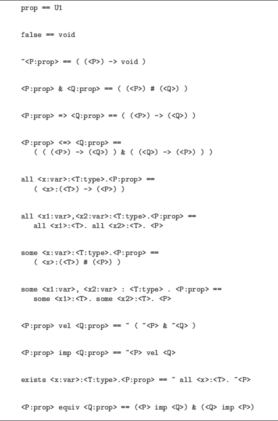
The basic logic definitions were discussed in chapter 3, but they are repeated in figure 11.1 for reference in the subsequent sections. To illustrate the kind of parenthesizing which it is wise to do in practice only white space has been added to the text of the actual library object.
Lists and Arrays
This section presents a few basic objects from list theory and array theory. We start with the idea of a discrete type, which is a type for which equality is decidable. Discreteness is required for the element comparisons that are needed, for example, in searching a list for a given element. Also, we need the idea that a proposition is decidable, i.e., that it is either true or false.
     discrete(<T:type>) ==
        all x,y:<T>. (x=y in <T>) | ~(x=y in <T>)
     < P: T->prop > is decidable on <T:type> ==
        all x:<T>. P(x) | ~P(x)
Figure 11.2 gives
two versions of the list head function,
which differ only on how they treat the empty list.
The theorem statements following each definition define the behavior
of the respective head function.
The definition of the tail function is straightforward.
=y in A\end{verbatim}
\vspace{2pt}
\hrule
\end{figure}](img802.png)
tl(<l:list>) == list_ind( <l>; nil; h,t,v. t )
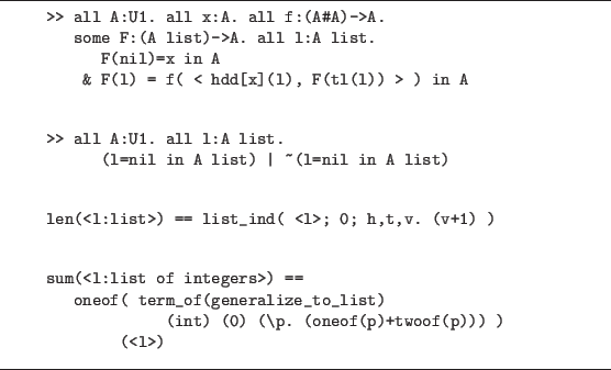
Given a function of
the appropriate type, the first theorem
(named ``generalize_ to_list'') listed in figure 11.3
specifies the construction of another function that iterates
the given function over a list. The object extracted from the
proof is used in a function which sums the elements of a list.
The definition of the membership predicate for lists uses a recursive proposition.
     <e:element> on <l:list> over <T:type> ==
        list_ind( <l>; void; h,t,v. (<e>=h in <T>) | v )
     >> all A:U1. all x:A. all l:A list.
           (x on L over A) in U1
The above type of use of list_ind to define a proposition is
common and is worth a bit of explanation.
Suppose that

this type (proposition) is inhabited (true) exactly when one of the
 is true.
The following is another example of a recursively defined proposition;
it defines a predicate over lists of a certain type which is true
of list ![]() exactly when
exactly when ![]() has no repeated elements.
has no repeated elements.
     <l:list> is nonrepetitious over <T:type> ==
        list_ind( <l>; one; h,t,v. ~(h on t over <T>) and v )
Given this definition, the following theorems are provable.
>> all A:U1. nil is nonrepetitious over A
     >> all A:U1. all x:A. all l:A list.
          ~(x on l over A) & l is nonrepetitious over A
          =>  x.l is nonrepetitious over A
The next theorem defines a function which searches an array for the first occurrence of an element with a given property. (Arrays are taken to be functions on segments of the integers.)
search:
     >> all A:U1. all n:int.
        all f:{1,...,n}->A. all P:A->prop.
           P is decidable on A
           => all k:int.
                 1<=k<=n
                 =>   all x:{1,...,k}. ~P(f(x))
                    | some x:{1,...,k}. P(f(x))
                        & all y:{1,...,x-1}. ~P(f(y))
|
Cardinality
This section presents some elementary facts from the theory of cardinality and discusses a proof of the familiar pigeonhole principle.11.1
Figure 11.4 lists the definitions and lemmas used to prove the pigeonhole principle.
lemma_wf_1 is used to prove well-formedness conditions that arise in the other lemmas. We use the lemma lemma_arith when we want to do a case analysis on an integer equality. lemma_hole finds for some f and some y in the codomain of f an x in the domain of f for which f(x)=y (or indicates if no such x can be found). This lemma can be considered as a computational procedure that will be useful in the proof of the main lemma, lemma_1. This lemma is a simplified version of the theorem, with the domain of f only one element larger than the range. The theorem pigeonhole_principle follows in short order from lemma_1.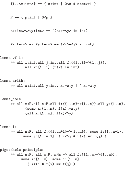
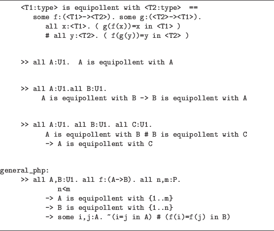
Using the pigeonhole principle one can prove a more general form of the principle. Figure 11.5 lists the definitions needed to state the theorem and the statement of the theorem.
The proof of lemma_hole is a straightforward induction on m, the size of the domain of f. It is left as an exercise.
We consider in depth the proof of lemma_1. In the proof given below we elide hypotheses which appear previously in order to condense the presentation. The system performs no such action. After introducing the quantifiers we perform induction on the eliminated set type n (we need to get an integer, n1 below, to do induction on). This induction is over the size of the domain and range together.
+----------------------------------------------------------+
|EDIT THM lemma_1                                          |
|----------------------------------------------------------|
|# top 1 2                                                 |
|1. n:P                                                    |
|2. n1:int                                                 |
|[3]. 0<n1                                                 |
|>> all f:({1..n1+1}->{1..n1}).some i:{1..n1+1}.           |
|   some j:{1..n1+1}.  (i<>j#f(i).=z.f(j))                 |
|                                                          |
|BY elim 2 new ih,k                                        |
|                                                          |
|1# {down case}                                            |
|                                                          |
|2* 1...3.                                                 |
|   >> all f:({1..0+1}->{1..0}).some i:{1..0+1}.           |
|      some j:{1..0+1}.  (i<>j#f(i).=z.f(j))               |
|                                                          |
|3# 1...3.                                                 |
|   4. k:int                                               |
|   5. 0<k                                                 |
|   6. ih:all f:({1..k-1+1}->{1..k-1}).some i:{1..k-1+1}.  |
|      some j:{1..k-1+1}.(i<>j#f(i).=z.f(j))               |
|   >> all f:({1..k+1}->{1..k}).some i:{1..k+1}.           |
|      some j:{1..k+1}.  (i<>j#f(i).=z.f(j))               |
|                                                          |
+----------------------------------------------------------+
|
The ``up'' case is the only interesting case. First we intro f, and then since we want to use the lemma lemma_hole a proper form of it is sequenced in and appears as hypothesis 9 below. We use this lemma on f:{1..k}->{1..k}. We then do a case analysis on the lemma.
The left case is trivial. We have some x such that f(x)=f(k+1), and x is in {1..k}, so x<>k; thus we can intro x for i and k+1 for j. Let us concentrate on the more interesting right case. Using our induction hypothesis requires a function f:{1..k}->{1..k-1}; our function will possibly map a value of the domain to k. We thus make a new function by taking the value of f that would have mapped to k to whatever k+1 maps to. Since by the hole lemma (hypothesis 10) no f(x) has the same value as f(k+1), our new function will just be a permutation of the old function.
+------------------------------------------------------------+
|EDIT THM lemma_1                                            |
-------------------------------------------------------------|
|# top 1 2 3 1 2 2 2                                         |
|1...6.                                                      |
|7. f:({1..k+1}->{1..k})                                     |
|8. all y:{1..k}. (some x:{1..k}.f(x).=z.y)                  |
|                |(all x:{1..k}.f(x)<>y)                     |
|9.  (some x:{1..k}.f(x).=z.f(k+1))                          |
|   |(all x:{1..k}.f(x)<>f(k+1))                             |
|10. (all x:{1..k}.f(x)<>f(k+1))                             |
|>> some i:{1..k+1}.some j:{1..k+1}.(i<>j#f(i).=z.f(j))      |
|                                                            |
|BY elim 6 on \x.int_eq(f(x);k;f(k+1);f(x))                  |
|                                                            |
|1# 1...10.                                                  |
|   >> \x.int_eq(f(x);k;f(k+1);f(x))                         |
|       in ({1..k-1+1}->{1..k-1})                            |
|                                                            |
|2# 1..10.                                                   |
|   11. i:({1..k-1+1})#(j:({1..k-1+1})#((i<>j)#              |
|         ((\x.int_eq(f(x);k;f(k+1);f(x)))(i)                |
|         =(\x.int_eq(f(x);k;f(k+1);f(x)))(j) in int)))      |
|   >> some i:{1..k+1}.some j:{1..k+1}.(i<>j#f(i).=z.f(j))   |
|                                                            |
+------------------------------------------------------------+
We can now unravel our induction hypothesis into hypotheses 12, 14, 16 and 17 below. We want to do a case analysis on f(i)=k | ~f(i)=k (hypothesis 18); we sequence this fact (proven by lemma_arith) in. Consider the case where f(i)=k. Then we can prove f(k+1)=f(j) by reducing hypothesis 17 (note how we have to sequence in 20 and 21, and then f(k+1)=f(j), in order to reduce the hypothesis).
+----------------------------------------------------------+
|EDIT THM lemma_1                                          |
|----------------------------------------------------------|
|# top 1 2 3 1 2 2 2 2 1 1 1 2 1 2 2                       |
|1. n:P                                                    |
|12. i:{1..k-1+1}                                          |
|14. j:{1..k-1+1}                                          |
|16. i<>j                                                  |
|17. (\x.int_eq(f(x);k;f(k+1);f(x)))(i)=                   |
         (\x.int_eq(f(x);k;f(k+1);f(x)))(j) in int         |
|18. f(i).=z.k|~f(i).=z.k                                  |
|19. f(i).=z.k                                             |
|20. (\x.int_eq(f(x);k;f(k+1);f(x)))(i)=f(k+1) in int      |
|21. (\x.int_eq(f(x);k;f(k+1);f(x)))(j)=f(j) in int        |
|>> some i:{1..k+1}.some j:{1..k+1}.(i<>j#f(i).=z.f(j))    |
|                                                          |
|BY (*combine 17,20,21*)                                   |
|   seq f(k+1)=f(j) in int                                 |
|                                                          |
|1* 1...19.                                                |
|   20. (\x.int_eq(f(x);k;f(k+1);f(x)))(i)=f(k+1) in int   |
|   21. (\x.int_eq(f(x);k;f(k+1);f(x)))(j)=f(j) in int     |
|   >> f(k+1)=f(j) in int                                  |
|                                                          |
|2# 1...21.                                                |
|   22. f(k+1)=f(j) in int                                 |
|   >> some i:{1..k+1}.some j:{1..k+1}.(i<>j#f(i).=z.f(j)) |
|                                                          |
+----------------------------------------------------------+
We can now prove our goal by letting i be k+1 and j be j. k+1<>j follows from hypothesis 14.
+-------------------------------------------------------+
|EDIT THM lemma_1                                       |
|-------------------------------------------------------|
|# top 1 2 3 1 2 2 2 2 1 1 1 2 1 2 2 2 2 2              |
|1...13.                                                |
|14. j:{1..k-1+1}                                       |
|15..22.                                                |
|>> (k+1 <>j#f(k+1 ).=z.f(j))                           |
|                                                       |
|BY intro                                               |
|   ....                                                |
|                                                       |
+-------------------------------------------------------+
|
This concludes this part of the proof. We now consider the other case, i.e., ~f(i)=k. If f(j)=k then the conclusion follows by symmetry from above (note that in the current system we still have to prove this; eventually a smart symmetry tactic could do the job). Otherwise, ~f(j)=k, and we can reduce hypothesis 17 to f(i)=f(j) as done previously (see hypotheses 22 and 23 below). The conclusion then follows from hypotheses 16 and 24.
+---------------------------------------------------+ |EDIT THM lemma_1 | |---------------------------------------------------| |* top 1 2 3 1 2 2 2 2 1 1 1 2 2 2 2 2 2 2 2 | |1...15. | |16. i<>j | |17. (\x.int_eq(f(x);k;f(k+1);f(x)))(i)= | | (\x.int_eq(f(x);k;f(k+1);f(x)))(j) in int | |18. f(i).=z.k|~f(i).=z.k | |19. ~f(i).=z.k | |20. f(j).=z.k|~f(j).=z.k | |21. ~f(j).=z.k | |22. (\x.int_eq(f(x);k;f(k+1);f(x)))(i)=f(i) in int | |23. (\x.int_eq(f(x);k;f(k+1);f(x)))(j)=f(j) in int | |24. f(i)=f(j) in int | |>> (i<>j#f(i).=z.f(j)) | | | |BY intro | | ... | | | +---------------------------------------------------+ |
This completes the proof of lemma_1. The proof of pigeonhole_principle is straightforward and is left as an exercise for the reader.
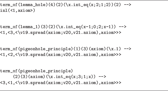
The evaluator, when applied to term_of(pigeonhole_principle) on a given function f, returns the i and j such that f(i)=f(j) and i<>j. Figure 11.6 gives some examples of such evaluations performed by the evaluator. The redex on the left of the -> evaluates to the contractum on the right of the ->.
Regular Sets
This section describes an existing library of theorems from the theory
of regular sets. The library was constructed in part to try out some
general-purpose tactics which had recently been written; the most useful
of these were the membership tactic (see chapter 9) and several
tactics which performed computation steps and definition
expansions
in goals. The membership tactic was able to prove all of the membership
subgoals which arose, i.e., all those of the form ![]() »
» ![]() in
in ![]() .
The
other tactics mentioned were heavily used but required a fair amount of
user involvement; for example, the user must explicitly specify which
definitions to expand.
Including planning, the total time required to construct the library and
finish all the proofs was about ten hours.
.
The
other tactics mentioned were heavily used but required a fair amount of
user involvement; for example, the user must explicitly specify which
definitions to expand.
Including planning, the total time required to construct the library and
finish all the proofs was about ten hours.
For the reader unfamiliar with the subject, this theory
involves a certain
class of computationally ``simple'' sets of words over some
given alphabet; the sets are those which can be built
from singleton sets using three operations, which are denoted by
![]() ,
, ![]() and
and ![]() . There should be enough
explanation in what follows to make the theorems understandable
to almost everyone.
. There should be enough
explanation in what follows to make the theorems understandable
to almost everyone.
We begin with a presentation of the library; a discussion of some of the objects will follow. This theory uses extractions for most of the basic objects. For example, the right-hand side of the definition for the function flatten is just term_of(flatten_)(<l>); the actual Nuprl term for the function is introduced in the theorem flatten_. As a convention in this theory, a DEF name with ``_'' appended is the name of the corresponding theorem that the defined object is extracted from. Figure 11.7 presents the first part of the library, which contains the definitions of the basic objects, such as basic list operations and the usual operations on regular sets. Objects not particular to this theory, such as the definitions of the logical connectives, are omitted. The alphabet over which our regular sets are formed is given the name E and is defined to be atom (although all the theorems hold for any type). The collection of words over E, E*, is defined to be the lists over E, and the regular sets for the purposes of this theory are identified with their meaning as subsets of E*:
E* == (E list)
R(E) == (E*->U1)
Note first that we have identified the subsets of E* with
the predicates over E*; for more on representing sets, see the preceding
chapter. This means that if 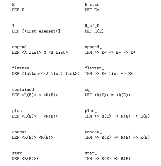
Figure 11.8 shows the next part of the library, which contains some lemmas expressing some elementary properties of the defined objects. It should be noted here that the theorems we are proving are identities involving the basic operations, and they are true over all subsets, not just the regular ones. This allows us to avoid cutting R(E) down to be just the regular sets, and we end up proving more general theorems. (It would be a straightforward matter to add this restriction by using a recursive type to define the regular expressions and defining an evaluation function.)
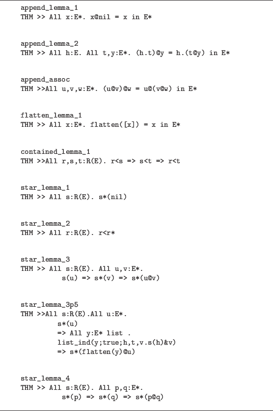
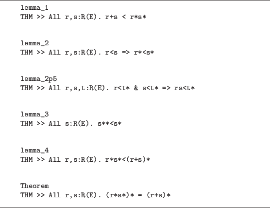
Figure 11.9 list some lemmas expressing properties of regular sets, and the main theorem of the library.
We now turn our attention to objects contained in the library. The following descriptions of library objects should give the flavor of the development of this theory. This proof top and DEF together give the definition of append.
     >> E* -> E* -> E*
     BY explicit intro \x.\y. list_ind(x;y;h,t,v.(h.v))
<l1:A list>@<l2:A list> == (term_of(append_)(<l1>)(<l2>))
We use append to define the function flatten, which
takes a list of lists and concatenates them:
     >> E* list -> E*
     BY explicit intro \x. list_ind(x;nil;h,t,v.h@v)
The definitions of containment, ``<'', and equality
are what one would expect, given the definition of regular sets.
<r1:R(E)> < <r2:R(E)> == All x:E*. (<r1>)(x) => (<r2>)(x)
<r1:R(E)> = <r2:R(E)> == <r1> < <r2> & <r2> < <r1>
The following three proof tops give the definitions of
     >> R(E) -> R(E) -> R(E)
     BY explicit intro \r.\s.\x. ( r(x) | s(x) )
     >> R(E)->R(E)->R(E)
     BY explicit intro
         \r.\s.\x. Some u,v:E*.
           u@v=x in E* & r(u) & s(v)
     >> R(E) -> R(E)
     BY explicit intro
         \r.\x. Some y:E* list.
           list_ind(y;true;h,t,v.r(h)&v)
           & flatten(y)=x in E*
Note the use of list_ind to
define
a predicate recursively.
The presentation concludes with a few shapshots that should
give an idea of what the proofs in this library are like.
First, consider a few steps of the proof of
star_lemma_3p5, which states that if ![]() is in set
is in set ![]() then for all sets of words in
then for all sets of words in ![]() the concatenation of all words in the set, followed by
the concatenation of all words in the set, followed by ![]() , is also in
, is also in ![]() . The major proof step, done
after the goal has been ``restated'' by
moving things into the hypothesis list, is induction on
the list y.
. The major proof step, done
after the goal has been ``restated'' by
moving things into the hypothesis list, is induction on
the list y.
,----------------------------------------------, |* top 1 1 1 | |1. s:(R(E)) | |2. u:(E*) | |3. (s*(u)) | |4. y:(E* list ) | |>> ( list_ind(y;true;h,t,v.s(h)&v) | | => s*(flatten(y)@u)) | | | |BY elim y new p,h,t | | | |1* 1...4. | | >> ( list_ind(nil;true;h,t,v.s(h)&v) | | => s*(flatten(nil)@u)) | | | |2* 1...4 | | 5. h:E* | | 6. t:(E* list ) | | 7. p:( list_ind(t;true;h,t,v.s(h)&v) | | => s*(flatten(t)@u)) | | >> ( list_ind(h.t;true;h,t,v.s(h)&v) | | => s*(flatten(h.t)@u)) | '----------------------------------------------' |
The first subgoal is disposed of by doing some computation steps on subterms of the consequent of the conclusion. The second subgoal is restated, and the last hypothesis is reduced using a tactic.
,-----------------------------------------------, |* top 1 1 1 2 1 | |1...7. | |8. ( list_ind(h.t;true;h,t,v.s(h)&v) ) | |>> ( s*(flatten(h.t)@u)) | | | |BY compute_hyp_type | | | |1* 1...7. | | 8. s(h)&list_ind(t;true;h,t,v.s(h)&v) | | >> ( s*(flatten(h.t)@u)) | '-----------------------------------------------' |
The rest of the proof is just a matter of expanding a few definitions and doing some trivial propositional reasoning.
Now consider Theorem. The proof is abstract with respect to the representation of regular sets; lemmas lemma_1 to lemma_4 and the transitivity of containment are all that is needed. First, the two major branches of the proof are set up.
,-----------------------------------------------, |* top 1 | |1. r:(R(E)) | |2. s:(R(E)) | |>> ( (r*s*)*=(r+s)*) | | | |BY intro | | | |1* 1...2. | | >> ((r*s*)*<(r+s)*) | | | |2* 1...2. | | >> ((r+s)*<(r*s*)*) | '-----------------------------------------------' |
The rest of the proof is just lemma application (using lemma application tactics); for example, the rule below is actually a definition whose right-hand side calls a tactic which computes from the goal the terms with which to instantiate the named lemma, and then attempts (successfully in this case) to finish the subproof.
+------------------------------------------+ |EDIT THM Theorem | |------------------------------------------| |* top 1 1 1 1 1 | |1. r:(R(E)) | |2. s:(R(E)) | |3. ( r*s*<(r+s)* => r*s**<(r+s)**) | |>> (r*s*<(r+s)* ) | | | |BY Lemma lemma_4 | | | +------------------------------------------+ |
Real Analysis
This section presents Nuprl formalizations of constructive versions of some of the most familiar concepts of real analysis. The account here is brief; more on this subject will be found in the forthcoming thesis of Howe [Howe 86].
We begin with a basic type of the positive integers, two definitions that make terms involving spread more readable and an alternative definition of some which uses the set type instead of the product.
     Pos ==
       {n:int|0<n}
     let <x:var>,<y:var>=<t:term> in <tt:term> ==
        spread(<t>;<x>,<y>.<tt>)
     let <w:var>,<x:var>,<y:var>,<z:var>=
                   <t1:term>,<t2:term> in <t3:term> ==
        let <w>,<x>=<t1> in let <y>,<z>=<t2> in <t3>
     Some <x:var>:<T:type> where <P:prop> ==
        { <x>:<T> | <P> }
Figure 11.10 lists a few of the standard definitions involved in the theory
of rationals. Note that the
rationals, Q, are
a quotient type; therefore, as explained in the
section on
quotients in chapter 10, we must use the squash operator
(||...||) in the definition of 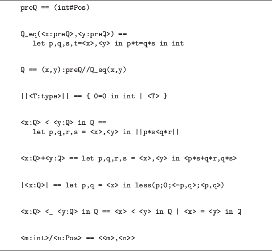
We adopt Bishop's formulation of the real
numbers as regular (as opposed to Cauchy)
sequences of rational numbers. With the regularity approach a real
number is just a sequence of rationals, and the regularity
condition (see the definition of R below) permits the
calculation of arbitrarily close rational
approximations to a given
real number. With the usual approach a real number would actually
have to be a pair comprising a sequence and a function giving the
convergence rate.
Figure 11.11 lists the definition of the reals and functions
and predicates involving the reals.
The definition of ![]() is a little different than
might be expected, since
it has some computational content, i.e., a positive lower
bound to the difference of the two real numbers.
is a little different than
might be expected, since
it has some computational content, i.e., a positive lower
bound to the difference of the two real numbers.
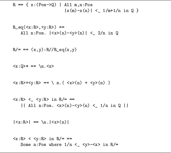
The definition of ![]() (<_) in figure 11.11 is
squashed since it is a predicate over a quotient type.
However, in the case of the real numbers the use of the squash
operator does not completely solve the problem with quotients.
For example,
if X is a discrete type (i.e., if equality in
X is decidable) then there are no nonconstant functions
in R/= -> X. In particular, the following basic facts fail to
hold.
(<_) in figure 11.11 is
squashed since it is a predicate over a quotient type.
However, in the case of the real numbers the use of the squash
operator does not completely solve the problem with quotients.
For example,
if X is a discrete type (i.e., if equality in
X is decidable) then there are no nonconstant functions
in R/= -> X. In particular, the following basic facts fail to
hold.
All x:R/=. All n:int. Some a:Q. |x-a| <_ 1/n in Q
All x,y,z:R/=. x<y in R/= => ( z<y in R/= | x<z in R/=)
We are therefore precluded from using the quotient type here
as an abstraction mechanism and will have to do most of
our work over R. R/= can still
be used, however,
to gain access to the substitution and equality rules, and it
is a convenient shorthand for expressing concepts involving
equality.
Consider the computational aspects of the next two definitions.
Knowing that a sequence of real
numbers converges involves
having the limit and the function which gives the convergence
rate. Notice that we have used the set type (in the
definition of some ![]() where) to isolate the computationally
interesting parts of the concepts.
where) to isolate the computationally
interesting parts of the concepts.
     <x:Pos->R> is Cauchy ==
         All k:Pos.
           Some M:Pos where
                  All m,n:Pos.
                     M <_ m in int => M <_ n in int =>
                     |<x>(m)-<x>(n)| <_ (1/k)* in R/=
     <x:Pos->R> converges ==
         Some x:R/=. All k:Pos.
           Some N:Pos where
                   All n:int. N <_ n in int =>
                      |(<x>)(n)-x| <_ (1/k)* in R/=
Figure 11.12 defines the ``abstract data type'' of compact
intervals.
Following is the (constructive) definition of continuity
on a compact interval. A function in R+ -> R+
which inhabits the type given as the definition of continuity
is called
a modulus of continuity.
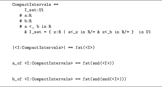
R+ == { x:R | 0<x in R/= }
     <f:|I|->R> continuous on <I:CompactIntervals> ==
        All eps:R+.
           Some del:R+ where All x,y:|<I>|.
           |x-y| <_ del in R/=  =>  |<f>(x)-<f>(y)| <_ eps
It is now a simple matter to state a constructive version of the
intermediate value theorem.
     >> All I:CompactIntervals. All f:|I|->R.
           f continuous on I  &  f(a_of I) < 0 in R
              &  0 < f(b_of I) in R
           => All eps:R+.
                 Some x:|I|. |f(x)| < eps in R
A proof of the theorem above will yield function resembling a
root-finding program.
Denotational Semantics
This section presents a constructive denotational semantics theory for a simple program language where meaning is given as a stream of states. The following definitions and theorems illustrate this library.
The data type Program is built from a dozen type definitions like those which follow.
Atomic_stmt == Abort | Skip | Assignment Program == (depth:N # Statement(depth))
Statement(<d>) ==
     ind(<d>; x,y.void; void; x,T. Atomic_stmt |
         (T#T) *concat* | (expr#T) *do loop* |
         expr#T#T *if then else*)
|
The type for stream of states, S, is defined below. Note that the ind form in the definition of Statement approximates a type of trees, while N->State approximates a stream of states. The intended meaning for S is that given an initial state, its value on n is the program state after executing n steps.
State* == Identifier -> Value
Done == {x:atom | x="done" in atom}
State    == State* | Done
<st:State> terminated ==
     decide(<st>; u.void; u.int)
S        ==
     {f: State -> N -> State |
     All a:State, n:N.
	f(a)(n) terminated => f(a)(n+1) terminated}
|
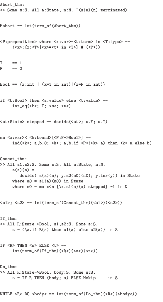
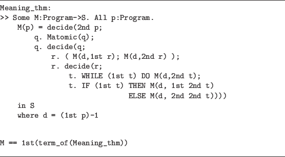
Figure 11.13 presents the various meaning functions as extracted objects. Using these definitions, one can define a meaning function, M, for programs. This is done in figure 11.14 in the definition of M, the meaning function for programs. With M one can reason about programs as well as executing them directly using the evaluation mechanism.
Footnotes
- ... principle.11.1
- This principle states that any function mapping a finite set into a smaller finite set must map some pair of elements in the domain to the same element in the codomain.