
The Book
Implementing Mathematics with The Nuprl Proof Development System
See title page for important information about this reference
Next: Statements and Definitions in Up: Index Previous: Overview Contents
- The Typed Lambda Calculus
- Extending the Typed Lambda Calculus
- Dependent Function Space
- Cartesian Product
- Dependent Products
- Disjoint Union
- Integers
- Atoms and Lists
- Equality and Propositions as Types
- Sets and Quotients
- Semantics
- Relationship to Set Theory
- Relationship to Programming Languages
Introduction to Type Theory
Sections 2.1 to 2.4 introduce a sequence of approximations to Nuprl, starting with a familiar formalism, the typed lambda calculus. These approximations are not exactly subsets of Nuprl, but the differences between these theories and subtheories of Nuprl are minor. These subsections take small steps toward the full theory and relate each step to familiar ideas. Section 2.5 summarizes the main ideas and can be used as a starting point for readers who want a brief introduction. The last two sections relate the idea of a type in Nuprl to the concept of a set and to the concept of a data type in programming languages.
The Typed Lambda Calculus
A type
is a collection of objects having similar
structure. For instance, integers,
pairs of integers and functions over integers are
at least three distinct types. In both mathematics
and programming the collection of functions is further subdivided
based on the kind of input for which the function makes sense, and these
divisons are also called types, following the vocabulary of the very
first type theories [Whitehead & Russell 25].
For example, we say that the integer successor function
is a function from integers to
integers,
that inversion is a function from invertible functions to functions
(as in ``subtraction is the inverse of addition''), and that the operation
of functional composition is a function from two functions to their composition.
One modern notation for the type of functions from type ![]() into type
into type ![]() is
is
![]() (read as
(read as ![]() ``arrow''
``arrow'' ![]() ).
Thus integer successor has type
).
Thus integer successor has type
![]() ,
and the curried form of the composition of integer
functions has type
,
and the curried form of the composition of integer
functions has type
![]() .
For our first look at types we will consider only those built from
type variables
.
For our first look at types we will consider only those built from
type variables ![]() using arrow.
Hence we will have
using arrow.
Hence we will have
![]() , etc.,
as types,
but not
, etc.,
as types,
but not
![]() .
This will allow us to examine the general properties of functions without
being concerned with the details of concrete types such as integers.
.
This will allow us to examine the general properties of functions without
being concerned with the details of concrete types such as integers.
One of the necessary steps in defining a type is choosing a notation for
its elements.
In the case of the integers, for instance, we use notations such as
![]() .
These are the defining notations, or canonical forms, of the type.
Other notations, such as
.
These are the defining notations, or canonical forms, of the type.
Other notations, such as ![]() ,
, ![]() and
and ![]() , are not
defining notations but are derived notations or noncanonical forms.
, are not
defining notations but are derived notations or noncanonical forms.
Informally, functions are named in a variety of ways.
We sometimes use special symbols like ![]() or
or ![]() .
Sometimes in informal mathematics one might abuse the notation and say
that
.
Sometimes in informal mathematics one might abuse the notation and say
that ![]() is the successor function.
Formally, however, we regard
is the successor function.
Formally, however, we regard ![]() as an ambiguous
value of the successor function and adopt a notation for the function
which distinguishes it from its values.
Betrand Russell [Whitehead & Russell 25] wrote
as an ambiguous
value of the successor function and adopt a notation for the function
which distinguishes it from its values.
Betrand Russell [Whitehead & Russell 25] wrote ![]() for the
successor function, while
Church [Church 51] wrote
for the
successor function, while
Church [Church 51] wrote ![]() .
Sometimes one sees the notation
.
Sometimes one sees the notation ![]() , where
, where ![]() is used as a ``hole'' for the
argument.
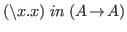
In Nuprl we adopt the lambda notation, using
is used as a ``hole'' for the
argument.
In Nuprl we adopt the lambda notation, using
![]() as a printable
approximation to
as a printable
approximation to ![]() .
This notation is not suitable for all of our needs, but it is an adequate
and familiar place to start.
.
This notation is not suitable for all of our needs, but it is an adequate
and familiar place to start.
A Formal System
We will now define a small formal system for deriving typing relations
such as
![]()
![]()
![]() .
To this end we have in mind the following two classes of expression.
A type expression has the form of a type variable
.
To this end we have in mind the following two classes of expression.
A type expression has the form of a type variable ![]() (an
example of an atomic type) or the form
(an
example of an atomic type) or the form
![]() , where
, where
![]() and
and ![]() are type expressions.
If we omit parentheses then arrow associates to the right; thus
are type expressions.
If we omit parentheses then arrow associates to the right; thus
![]() is
is
![]() .
An object expression has the form of a variable,
.
An object expression has the form of a variable, ![]() , an
abstraction,
, an
abstraction,
![]() or of an application,
or of an application, ![]() , where
, where ![]() and
and ![]() are
object expressions.
We say that
are
object expressions.
We say that ![]() is the body
of
is the body
of
![]() and the scope of
and the scope of ![]() , a
binding operator.
, a
binding operator.
In general, a variable ![]() is bound in a term
is bound in a term ![]() if
if ![]() has a subterm of
the form
has a subterm of
the form
![]() .
Any occurrence of
.
Any occurrence of ![]() in
in ![]() is bound.
A variable occurrence in
is bound.
A variable occurrence in ![]() which is not bound is called free.
We say that a term
which is not bound is called free.
We say that a term ![]() is free for a variable
is free for a variable ![]() in a term
in a term ![]() as long as no
free variable of
as long as no
free variable of ![]() becomes bound when
becomes bound when ![]() is substituted for each free
occurrence of
is substituted for each free
occurrence of ![]() . For example,
. For example, ![]() is free for
is free for ![]() in
in
![]() , but
, but ![]() is not.
If
is not.
If ![]() has a free variable which becomes bound as a result of a substitution
then we say that the
variable has been captured.
Thus
has a free variable which becomes bound as a result of a substitution
then we say that the
variable has been captured.
Thus ![]() ``captures''
``captures'' ![]() if we try to substitute
if we try to substitute ![]() for
for ![]() in
in
![]() .
If
.
If ![]() is a term then
is a term then ![$t[a/x]$](img82.png) denotes the term which results from replacing
each free occurrence of
denotes the term which results from replacing
each free occurrence of ![]() in
in ![]() by
by ![]() ,
provided that
,
provided that ![]() is free for
is free for ![]() in
in ![]() .
If
.
If ![]() is not free for
is not free for ![]() then denotes
then denotes ![]() with
with ![]() replacing each
free
replacing each
free ![]() and the bound variables of
and the bound variables of ![]() which would capture free variables of
which would capture free variables of
![]() being renamed to prevent capture.
being renamed to prevent capture.
![$t[a_1,\ldots ,a_n/x_1, \ldots ,x_n]$](img83.png) denotes the simultaneous substitution of
denotes the simultaneous substitution of ![]() for
for ![]() .
We agree that two terms which differ only in their bound variable
names will be treated as equal everywhere in the theory, so
will denote the same term inside the theory regardless of
capture.
Thus, for example,
.
We agree that two terms which differ only in their bound variable
names will be treated as equal everywhere in the theory, so
will denote the same term inside the theory regardless of
capture.
Thus, for example,
![$(\backslash y.x(y))[t/x]$](img86.png) =
=
![]() and
and
![$(\backslash x.x(y))[t/x]$](img88.png) =
=
![]() and
and
![$(\backslash y.x(y))[y/x]$](img90.png) =
=
![]() .
.
When we write
 we mean that
![]() names a
function whose type is
names a
function whose type is
![]() .
To be more explicit about the role of
.
To be more explicit about the role of ![]() , namely that it
is a type variable,
we declare
, namely that it
is a type variable,
we declare ![]() in a context or environment.
The environment has the single declaration
in a context or environment.
The environment has the single declaration ![]() , which is read
``
, which is read
``![]() is a type.''2.1
is a type.''2.1
For ![]() a type expression and
a type expression and ![]() an object expression,
an object expression,  will be called
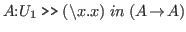
a typing. To separate the context from the typing we use ».
To continue the example above,
the full expression of our goal is
will be called
a typing. To separate the context from the typing we use ».
To continue the example above,
the full expression of our goal is
 .
.
In general we use the following terminology.
Declarations are either type declarations, in which
case they have the form ![]() , or object declarations, in
which case they have the form
, or object declarations, in
which case they have the form ![]() for
for ![]() a type expression.2.2A hypothesis list has the form of a sequence of declarations; thus,
for instance,
a type expression.2.2A hypothesis list has the form of a sequence of declarations; thus,
for instance,
![]() is a hypothesis list.
In a proper hypothesis list the types referenced in object declarations
are declared first (i.e., to the left of the object declaration).
A typing
has the form , where
is a hypothesis list.
In a proper hypothesis list the types referenced in object declarations
are declared first (i.e., to the left of the object declaration).
A typing
has the form , where ![]() is an object expression and
is an object expression and
![]() is a type expression.
A goal has the form
is a type expression.
A goal has the form
 ,
where
,
where ![]() is a hypothesis list and
is a typing.
is a hypothesis list and
is a typing.
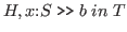
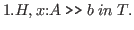
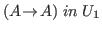
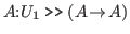
We will now give rules for proving goals. The rules specify a finite number of subgoals needed to achieve the goal. The rules are stated in a ``top-down'' form or, following Bates [Bates 79], refinement rules. The general shape of a refinement rule is:
goal by
- 1.
- subgoal 1
- .
- .
- .
- n.
- subgoal n.
Here is a sample rule.

It reads as follows: to prove that
![]() is a function in
is a function in
![]() in the
context
in the
context ![]() (or from hypothesis list
(or from hypothesis list ![]() ) we must achieve the subgoals
) we must achieve the subgoals
 and
and
 . That is, we must
show that the body
of the function has the type
. That is, we must
show that the body
of the function has the type ![]() under the assumption that the free variable
in the body has type
under the assumption that the free variable
in the body has type ![]() (a proof of this will demonstrate that
(a proof of this will demonstrate that ![]() is a
type expression), and that
is a
type expression), and that ![]() is a type expression.
is a type expression.
A proof is a finite tree whose nodes are pairs consisting of a subgoal and a rule name or a placeholder for a rule name. The subgoal part of a child is determined by the rule name of the parent. The leaves of a tree have rule parts that generate no subgoals or have placeholders instead of rule names. A tree in which there are no placeholders is complete. We will use the term proof to refer to both complete and incomplete proofs.
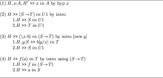
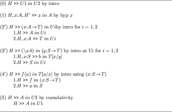
Figure 2.1 gives the rules for the small theory. Note that in rule (3) the square brackets indicate an optional part of the rule name; if the new y part is missing then the variable x is used, so that subgoal 1 is
The ``new variable'' part of a rule name allows the user to rename variables so as to prevent capture.
We say that an initial goal has the form
where the,
Figure 2.2 describes a complete proof of a simple fact.
This proof provides simultaneously a derivation of
 ,
showing that
,
showing that
![]() is a type expression; a derivation of
is a type expression; a derivation of
![]() , showing that this is an
object expression; and type information about all
of the subterms, e.g.,
, showing that this is an
object expression; and type information about all
of the subterms, e.g.,
There is a certain conceptual economy in providing all of this information in one format, but the price is that some of the information is repeated unnecessarily. For example, we show thatis in
;
is in
;
is in
;
is in
 three separate times.
This is an inherent difficulty with the style of ``simultaneous proof''
adopted in Nuprl.
In chapter 10 we discuss ways of minimizing its negative effects;
for example,
one could prove
three separate times.
This is an inherent difficulty with the style of ``simultaneous proof''
adopted in Nuprl.
In chapter 10 we discuss ways of minimizing its negative effects;
for example,
one could prove
 once as a lemma and
cite it as necessary, thereby sparing some repetition.
once as a lemma and
cite it as necessary, thereby sparing some repetition.
It is noteworthy that from a complete proof from an initial
goal of the form
we know that ![]() is a closed object
expression (one with no free variables) and
is a closed object
expression (one with no free variables) and ![]() is a type expression whose
free variables are declared in
is a type expression whose
free variables are declared in ![]() .
Also, in all hypotheses lists in all subgoals any expression appearing
on the right side of a declaration is either
.
Also, in all hypotheses lists in all subgoals any expression appearing
on the right side of a declaration is either ![]() or a type
expression whose variables are declared to the left.
Moreover, all
free variables of the conclusion in any subgoal are declared exactly
once in the corresponding hypothesis list.
In fact, no variable is declared at a subgoal unless it is free
in the conclusion.
Furthermore, every subterm
or a type
expression whose variables are declared to the left.
Moreover, all
free variables of the conclusion in any subgoal are declared exactly
once in the corresponding hypothesis list.
In fact, no variable is declared at a subgoal unless it is free
in the conclusion.
Furthermore, every subterm ![]() receives a type in
a subproof
receives a type in
a subproof
 , and in an application,
 ![]() ,
, ![]() will
receive a type
will
receive a type
![]() and
and ![]() will receive the type
will receive the type ![]() .
Properties of this variety can be proved by induction on
the construction of a complete proof.
For full Nuprl many properties like these are proved in the
Ph.D. theses of R. W. Harper [Harper 85] and S. F. Allen [Allen 86].
.
Properties of this variety can be proved by induction on
the construction of a complete proof.
For full Nuprl many properties like these are proved in the
Ph.D. theses of R. W. Harper [Harper 85] and S. F. Allen [Allen 86].
Computation System
The meaning of lambda terms
![]() is given by computation rules.
The basic rule,
called beta reduction,
is that
is given by computation rules.
The basic rule,
called beta reduction,
is that
![]() reduces to
reduces to ![$b[a/x]$](img133.png) ; for example,
; for example,
![]() reduces to
reduces to
![]() .
The strategy for computing applications
.
The strategy for computing applications ![]() is involves reducing
is involves reducing
![]() until it has the form
until it has the form
![]() ,
then computing
,
then computing
![]() .
This method of computing with noncanonical forms
.
This method of computing with noncanonical forms ![]() is called
head reduction or lazy evaluation, and
it is not the only possible way to compute.
For example, we might reduce
is called
head reduction or lazy evaluation, and
it is not the only possible way to compute.
For example, we might reduce ![]() to
to
![]() and then continue
to perform reductions in the body
and then continue
to perform reductions in the body ![]() .
Such steps might constitute computational optimizations of functions.
Another possibility is to reduce
.
Such steps might constitute computational optimizations of functions.
Another possibility is to reduce ![]() first until it reaches canonical
form before performing the beta reductions.
This corresponds to call-by-value computation
in a programming language.
first until it reaches canonical
form before performing the beta reductions.
This corresponds to call-by-value computation
in a programming language.
In Nuprl we use lazy evaluation, although for the simple calculus of typed lambda terms it is immaterial how we reduce. Any reduction sequence will terminate--this is the strong normalization result [Tait 67,Stenlund 72]--and any sequence results in the same value according to the Church-Rosser theorem [Church 51,Stenlund 72]. Of course, the number of steps taken to reach this form may vary considerably depending on the order of reduction.
Extending the Typed Lambda Calculus
Dependent Function Space
It is very useful to be able to describe functions whose range type
depends on the input.
For example, we can imagine a function on integers of the
form
![]() .
The type of this function on input
.
The type of this function on input ![]() is
is
![]() .
Call this type expression
.
Call this type expression ![]() ;
then the function type we want is written
;
then the function type we want is written
![]() and
denotes those functions
and
denotes those functions ![]() whose value on input
whose value on input ![]() belongs to
belongs to
![]() (
(
 ).
).
In the general case of pure functions we can introduce such types by
allowing declarations of parameterized types or, equivalently,
type-valued functions.
These are declared as
![]() .
To introduce these properly we must think of
.
To introduce these properly we must think of ![]() itself as a type,
but a large type.
We do not want to say
itself as a type,
but a large type.
We do not want to say
 to express that
 ![]() is a type
because this leads to paradox in the full theory. It is in the
spirit of type theory to introduce another layer of object, or in
our terminology, another ``universe'', called
is a type
because this leads to paradox in the full theory. It is in the
spirit of type theory to introduce another layer of object, or in
our terminology, another ``universe'', called ![]() .
In addition to the types in
.
In addition to the types in ![]() ,
, ![]() contains so-called large types,
namely
contains so-called large types,
namely ![]() and
types built from it
such as
and
types built from it
such as
![]() ,
,
![]() ,
,
![]() and so forth. To
say that
and so forth. To
say that ![]() is a large type we write
is a large type we write
 .
The new formal system allows the same class of object
expressions but a wider class of types.
Now a variable
.
The new formal system allows the same class of object
expressions but a wider class of types.
Now a variable ![]() is a type expression, the constant
is a type expression, the constant ![]() is a type expression, if
is a type expression, if ![]() is a type expression (possibly
containing a free occurrence of the variable
is a type expression (possibly
containing a free occurrence of the variable ![]() of type
of type ![]() ) then
) then
![]() is a type expression, and if
is a type expression, and if
![]() is an object expression of type
is an object expression of type
![]() then
then ![]() is
a type expression.
The old form of function space results when
is
a type expression.
The old form of function space results when ![]() does not
depend on
does not
depend on ![]() ;
in this case we still write
;
in this case we still write
![]() .
.
The new rules are listed in figure 2.3. With these rules we can prove the following goals.

With the new degree of expressiveness permitted by
the dependent arrow we are able to dispense with the hypothesis list in
the initial goal in the above examples.
We now say that an initial goal has the form
[0]
 , where
 ![]() is an object expression and
is an object expression and ![]() is a type expression.
One might expect that it would be more convenient to allow a
hypothesis list such as
is a type expression.
One might expect that it would be more convenient to allow a
hypothesis list such as
![]() , but such a list
would have to be checked to guarantee well-formedness of
the types.
Such checks become elaborate with types of the form
, but such a list
would have to be checked to guarantee well-formedness of
the types.
Such checks become elaborate with types of the form
![]() , and the
hypothesis-checking methods
would become as complex as the proof system itself.
As the theory is enlarged it will become impossible to provide an
algorithm which will guarantee the well-formedness of
hypotheses.
Using the proof system to show well-formedness will guarantee that
the hypothesis list is well-formed.
, and the
hypothesis-checking methods
would become as complex as the proof system itself.
As the theory is enlarged it will become impossible to provide an
algorithm which will guarantee the well-formedness of
hypotheses.
Using the proof system to show well-formedness will guarantee that
the hypothesis list is well-formed.
Hidden in the explanation above is a subtle point which affects
the basic design of Nuprl. The definition of a type expression
involves the clause ``![]() is an expression of type
is an expression of type
![]() .''
Thus, in order to know that is an allowable initial
goal, we may have to determine that a subterm of
.''
Thus, in order to know that is an allowable initial
goal, we may have to determine that a subterm of ![]() is of a
certain type; in the example above, we must show that
is of a
certain type; in the example above, we must show that
![]() is of type
is of type
![]() .
To define this concept precisely we would need some precise
definition of the relation that
.
To define this concept precisely we would need some precise
definition of the relation that ![]() is of type
is of type
![]() .
This could
be given by a type-checking algorithm or by an inductive definition,
but in either case the definition would be as complex as the proof
system that it is used to define.
.
This could
be given by a type-checking algorithm or by an inductive definition,
but in either case the definition would be as complex as the proof
system that it is used to define.
Another approach to this situation is to take a simpler definition
of an initial goal and let the proof system take care of ensuring
that only type expressions can appear on the right-hand side of
a typing. To this end, we define the syntactically simple concept of
a readable expression and then state that an initial goal has the
form
 , where
 ![]() and
and ![]() are these simple expressions.
Using this approach, an expression is either:
are these simple expressions.
Using this approach, an expression is either:
- a variable:
-
 ;
;
- a constant:
 ;
;
- an application:
 ;
;
- an abstraction:
-
 ; or
; or
- an arrow:
-
 ,
,
is proved then
Cartesian Product
One of the most basic ways of building new objects
in mathematics and programming involves the
ordered pairing constructor.
For example, in mathematics one builds rational numbers
as pairs of integers and complex numbers as pairs of reals.
In programming, a data processing record might
consist of a name paired with basic information
such as age, social security number, account
number and value of the account, e.g.,
![]() .
This item might be thought of as a single 5-tuple
or as compound pair
.
This item might be thought of as a single 5-tuple
or as compound pair
![]() .
In Nuprl we write
.
In Nuprl we write ![]() for the pair
consisting of
for the pair
consisting of ![]() and
and ![]() ;
;
![]() -tuples are built from pairs.
-tuples are built from pairs.
The rules for pairs are simpler than those for functions
because the canonical notations are built in a
simple way from components.
We say that ![]() is a canonical value for elements
of the type of pairs;
the name
is a canonical value for elements
of the type of pairs;
the name ![]() is canonical even if
is canonical even if ![]() and
and ![]() are not
canonical.
If
are not
canonical.
If ![]() is in type
is in type ![]() and
and ![]() is in type
is in type ![]() then
the type of pairs is written
then
the type of pairs is written ![]() and is called
the cartesian product.
The Nuprl notation is very similar to the set-theoretic notation,
where a cartesian product is written
and is called
the cartesian product.
The Nuprl notation is very similar to the set-theoretic notation,
where a cartesian product is written
![]() ; we choose
; we choose ![]() as the operator because it is
a standard ASCII character while
as the operator because it is
a standard ASCII character while ![]() is not.
In programming languages one might denote the
cartesian product as
is not.
In programming languages one might denote the
cartesian product as ![]() , as in the Pascal
record type, or as
, as in the Pascal
record type, or as ![]() , as in Algol 68 structures.
, as in Algol 68 structures.
The pair decomposition rule is the only Nuprl rule for products that is not as
one might expect from cartesian products in
set theory or from record types in programming.
One might expect operations, say ![]() and
and
![]() , obeying
, obeying
Instead of this notation we use a single form that generalizes both forms. One reason for this is that it allows a single form which is the inverse of pairing. Another more technical reason will appear when we discuss dependent products below. The form isand
where,
and
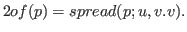
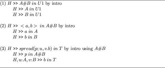
Figure 2.4 lists the rules for cartesian product. These rules allow us to assign types to pairs and to the spread terms. We will see later that Nuprl allows variations on these rules.
Dependent Products
Just as the function space constructor is generalized
from
![]() to
to
![]() , so too can the product
constructor be generalized to
, so too can the product
constructor be generalized to ![]() , where
, where ![]() can depend on
can depend on ![]() .
For example, given the declarations
.
For example, given the declarations
![]() and
and
![]() ,
, ![]() is a type in
is a type in ![]() .
The formation rule for dependent types becomes the following.
.
The formation rule for dependent types becomes the following.

The introduction rules change as follows.
![\(
(2') H \;\mbox{\tt >>}\;<a,b> \;in\;(x:A\char93 B) \mbox{ by intro}\\
\mb...
... \ \ \ }\mbox{\ \ \ \ }H, u:A,v:B[u/x] \;\mbox{\tt >>}\;b \;in\;T[<u,v>/z]\\
\)](img191.png)
The term ``over ![]() '' is needed in order to specify the substitution
of
'' is needed in order to specify the substitution
of ![]() in
in ![]() .
.
Disjoint Union
A
union operator represents another basic way of combining concepts.
For example, if ![]() represents the type of
triangles,
represents the type of
triangles, ![]() the type of rectangles and
the type of rectangles and ![]() the
type of circles, then we can say that an object is a
triangle or a rectangle or a circle by saying that
it belongs to the type
the
type of circles, then we can say that an object is a
triangle or a rectangle or a circle by saying that
it belongs to the type ![]() or
or ![]() or
or ![]() .
In Nuprl this type is written
.
In Nuprl this type is written
![]() .
.
In general if ![]() and
and ![]() are types, then so is their
disjoint union,
are types, then so is their
disjoint union, ![]() .
Semantically, not only is the union disjoint, but given an
element of
.
Semantically, not only is the union disjoint, but given an
element of ![]() , it must be possible to decide
which component it is in.
Accordingly, Nuprl uses the
canonical forms
, it must be possible to decide
which component it is in.
Accordingly, Nuprl uses the
canonical forms ![]() and
and ![]() to
denote elements of the union; for
to
denote elements of the union; for 
![]() is in
is in ![]() ,
and for
,
and for 
![]() is in
is in ![]() .
.
To discriminate on disjuncts, Nuprl uses
the form
![]() .
The interpretation is that if
.
The interpretation is that if ![]() denotes terms
of the form
denotes terms
of the form ![]() then
then
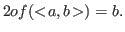
and if it denotes terms of the form![$decide(inl(a);u.e.;v.f) = \mbox{$e[a/u]$},$](img204.png)
The variable![$decide(inr(b);u.e;v.f) = \mbox{$f[b/v]$}.$](img205.png)
Integers
The type of integers, ![]() , is built
into Nuprl.
The canonical members of this type are
, is built
into Nuprl.
The canonical members of this type are
![]() .
The operations of addition,
.
The operations of addition, ![]() , subtraction,
, subtraction, ![]() ,
multiplication,
,
multiplication, ![]() , and division,
, and division, ![]() , are built into
the theory along with the modulus operation,
, are built into
the theory along with the modulus operation, ![]() ,
which gives the positive remainder of dividing
,
which gives the positive remainder of dividing ![]() by
by ![]() .
Thus
.
Thus
![]() .
Division of two integers produces the integer
part of real number division, so
.
Division of two integers produces the integer
part of real number division, so ![]() .
For nonnegative integers
.
For nonnegative integers ![]() and
and ![]() we have
we have
![]() .
.
There are three noncanonical forms associated
with the integers.
The first form captures the fact that integer
equality is decidable;
![]() denotes
denotes ![]() if
if
![]() and denotes
and denotes ![]() otherwise.
The second form captures the computational meaning
of less than;
otherwise.
The second form captures the computational meaning
of less than; ![]() denotes
denotes ![]() if
if ![]() and
and
![]() otherwise.
The third form provides
a mechanism for definition and proof by induction and is written
otherwise.
The third form provides
a mechanism for definition and proof by induction and is written
![]() .
It is easiest to see this form as a combination of two
simple induction forms over the nonnegative and nonpositive
integers.
Over the nonnegative integers (
.
It is easiest to see this form as a combination of two
simple induction forms over the nonnegative and nonpositive
integers.
Over the nonnegative integers (
![]() ) the form
denotes an inductive definition satisfying the following equations:
) the form
denotes an inductive definition satisfying the following equations:
Over the nonpositive integers (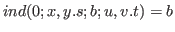
.
For example, this form could be used to define
.
In the form
![]()
![]() represents the integer argument,
represents the integer argument, ![]() represents the value of
the form if
represents the value of
the form if ![]() ,
, ![]() represents the inductive case for negative
integers, and
represents the inductive case for negative
integers, and ![]() represents the inductive case for positive
integers.
The variables
represents the inductive case for positive
integers.
The variables ![]() and
and ![]() are bound in
are bound in ![]() , while
, while ![]() and
and ![]() are bound in
are bound in ![]() .
.
Atoms and Lists
The type of atoms is provided in order to model character
strings.
The canonical elements of the type ![]() are ``...'', where ... is any character string.
Equality on atoms is decidable using the
noncanonical form
are ``...'', where ... is any character string.
Equality on atoms is decidable using the
noncanonical form
![]() , which denotes
, which denotes ![]() when
when
 and
and ![]() otherwise.
otherwise.
Nuprl also provides the type of lists over any other type ![]() ;
it is denoted
;
it is denoted ![]() .
The canonical elements of the type
.
The canonical elements of the type ![]() are
are ![]() , which
corresponds to the empty list, and
, which
corresponds to the empty list, and ![]() ,
where
,
where ![]() is in
is in ![]() and
and ![]() is in
is in ![]() .
For example, the list of the first three positive
integers in descending order is denoted
.
For example, the list of the first three positive
integers in descending order is denoted ![]() .
.
It is customary in the theory of lists to have head and tail functions such that
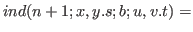
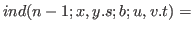
These and all other functions on lists that are built inductively are defined in terms of the list induction formand
.
With this form the tail function can be defined as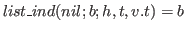
![$list\_ ind(a.r;b;h,t,v.t) = t[a,r,list\_ ind(r;b;h,t,v.t)/h,t,v]$](img245.png)
Equality and Propositions as Types
So far we have talked exclusively about types and their
members.
We now want to talk about simple declarative statements.
In the case of the integers many interesting facts
can be expressed as equations between terms.
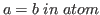
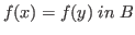
For example, we can say that a number ![]() is even by
writing
is even by
writing
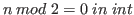 .
In Nuprl the equality relation on
.
In Nuprl the equality relation on ![]() is built-in;
we write
is built-in;
we write
 .
In fact, each type
.
In fact, each type ![]() comes with an equality relation
written
comes with an equality relation
written
 .
The idea that types come equipped with an equality
relation is very explicit in the writings of
Bishop [Bishop 67].
For example, in The Foundation of Constructive Analysis,
he says,
``A set is defined by describing what must be
done to construct an element of the set, and what must be
done to show that two elements of the set are equal.''
The notion that types come with an equality is central
to Martin-Löf's type theories as well.
.
The idea that types come equipped with an equality
relation is very explicit in the writings of
Bishop [Bishop 67].
For example, in The Foundation of Constructive Analysis,
he says,
``A set is defined by describing what must be
done to construct an element of the set, and what must be
done to show that two elements of the set are equal.''
The notion that types come with an equality is central
to Martin-Löf's type theories as well.
The equality relations
play a dual role in
Nuprl in that they can be used to express type membership relations
as well as equality relations within a type.
Since each type comes with such a relation, and since
 is a sensible relation only if
 ![]() and
and ![]() are
members of
are
members of ![]() , it is possible to express the idea that
, it is possible to express the idea that ![]() belongs to
belongs to ![]() by saying that
by saying that
 is true.
In fact, in Nuprl the form is really shorthand for
.
is true.
In fact, in Nuprl the form is really shorthand for
.
The equality statement
has the curious property
that it is either true or nonsense.
If ![]() has type
has type ![]() then is true; otherwise,
is not a sensible statement because is sensible only if
then is true; otherwise,
is not a sensible statement because is sensible only if
![]() and
and ![]() belong to
belong to ![]() .
Another way to organize type theory is to use a
separate form of judgement to say that
.
Another way to organize type theory is to use a
separate form of judgement to say that ![]() is in
a type, that is, to regard as distinct from
.
That is the approach taken by Martin-Löf.
It is also possible to organize type theory without
built-in equalities at all except for the most
primitive kind.
We only need equality on some two-element type,
say a type of booleans,
is in
a type, that is, to regard as distinct from
.
That is the approach taken by Martin-Löf.
It is also possible to organize type theory without
built-in equalities at all except for the most
primitive kind.
We only need equality on some two-element type,
say a type of booleans,
![]() ;
we could then define equality on
;
we could then define equality on ![]() as a function from
as a function from
![]() into
into
![]() The fact that each type comes equipped with equality
complicates an understanding of the rules,
as we see when we look at functions.
If we define a function
The fact that each type comes equipped with equality
complicates an understanding of the rules,
as we see when we look at functions.
If we define a function
 then
we expect that if
then
we expect that if
 then
then
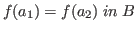 .
This is a key property of functions, that they respect
equality.
In order to guarantee this property there are
a host of rules of the form that if part of an
expression is replaced by an equal part then the results
are equal.
For example, the following are rules.
.
This is a key property of functions, that they respect
equality.
In order to guarantee this property there are
a host of rules of the form that if part of an
expression is replaced by an equal part then the results
are equal.
For example, the following are rules.

Propositions as Types
An equality form such as
makes sense
only if ![]() is a type
and
is a type
and ![]() and
and ![]() are elements of that type.
How should we express
the idea that
is well-formed?
One possibility is to use the same format as in
the case of types.
We could imagine a rule of the following form.
are elements of that type.
How should we express
the idea that
is well-formed?
One possibility is to use the same format as in
the case of types.
We could imagine a rule of the following form.

This rule expresses the right ideas, and it allows
well-formedness to be treated through the proof
mechanism in the same way that well-formedness is treated for types.
In fact, it is clear
that such an approach will be necessary for equality
forms if it is necessary for types because it is
essential to know that the ![]() in
is
well-formed.
in
is
well-formed.
Thus an adequate deductive apparatus is at hand for
treating the well-formedness of equalities, provided
that we treat
as a type.
Does this make sense on other grounds as well?
Can we imagine an equality as denoting a type?
Or should we introduce a new category, called Prop for proposition,
and prove
 ) in Prop?
The constructive interpretation of truth of any
proposition
) in Prop?
The constructive interpretation of truth of any
proposition ![]() is that
is that ![]() is provable.
Thus it is perfectly sensible to regard a
proposition
is provable.
Thus it is perfectly sensible to regard a
proposition ![]() as the type of its proofs.
For the case of an equality we make the
simplifying assumption that we are not
interested in the details of such proofs because
those details do not convey any more computational
information than is already contained in the
equality form itself.
It may be true that there are many ways to prove
, and
some of these may involve complex inductive
arguments.
However, these arguments carry
only ``equality information,'' not computational information,
so for simplicity we agree that equalities
considered as types are either empty if they
are not true or contain a single element, called
as the type of its proofs.
For the case of an equality we make the
simplifying assumption that we are not
interested in the details of such proofs because
those details do not convey any more computational
information than is already contained in the
equality form itself.
It may be true that there are many ways to prove
, and
some of these may involve complex inductive
arguments.
However, these arguments carry
only ``equality information,'' not computational information,
so for simplicity we agree that equalities
considered as types are either empty if they
are not true or contain a single element, called
![]() , if they are true.2.4
, if they are true.2.4
Once we agree to treat equalities as types
(and over ![]() , to treat
, to treat ![]() as a type also) then a remarkable
economy in the logic is possible.
For instance, we notice that the cartesian product
of equalities, say
as a type also) then a remarkable
economy in the logic is possible.
For instance, we notice that the cartesian product
of equalities, say
 , acts
precisely as the conjunction
, acts
precisely as the conjunction
 .
Likewise the disjoint union,
.
Likewise the disjoint union,
 ,
acts exactly like the constructive disjunction.
Even more noteworthy is the fact that the dependent product,
say
,
acts exactly like the constructive disjunction.
Even more noteworthy is the fact that the dependent product,
say
 , acts exactly like the
constructive existential quantifier,
, acts exactly like the
constructive existential quantifier,
 .
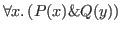
Less obvious, but also valid, is the interpretation
of
.
Less obvious, but also valid, is the interpretation
of
 as the universal statement,
 .
.
We can think of the types built up
from equalities (and inequalities in the case of integer)
using ![]() ,
, ![]() and
and
![]() as propositions, for
the meaning of the type constructors corresponds
exactly to that of the logical operators considered
constructively. As another example of this, if
as propositions, for
the meaning of the type constructors corresponds
exactly to that of the logical operators considered
constructively. As another example of this, if ![]() and
and ![]() are propositions then
are propositions then
![]() corresponds exactly
to the constructive interpretation of
corresponds exactly
to the constructive interpretation of
![]() .
That is, proposition
.
That is, proposition ![]() implies proposition
implies proposition ![]() constructively if and only if there is a method of
building a proof of
constructively if and only if there is a method of
building a proof of ![]() from a proof of
from a proof of ![]() ,
which is the case if and only if there is a function
,
which is the case if and only if there is a function ![]() mapping proofs of
mapping proofs of ![]() to proofs of
to proofs of ![]() .
However, given that
.
However, given that ![]() and
and ![]() are types such an
are types such an ![]() exists exactly when the
type
exists exactly when the
type
![]() is inhabited, i.e., when there is an element of
type
is inhabited, i.e., when there is an element of
type
![]() .
.
It is therefore sensible to treat propositions as types. Further discussion of this principle appears in chapters 3 and 11.
Is it sensible to consider any type, say ![]() or
or ![]() ,
as a proposition?
Does it make sense to assert
,
as a proposition?
Does it make sense to assert ![]() ?
We can present the logic and the type theory in a
uniform way if we agree to take the basic form of
assertion as ``type
?
We can present the logic and the type theory in a
uniform way if we agree to take the basic form of
assertion as ``type ![]() is inhabited.''
Therefore, when we write the goal
is inhabited.''
Therefore, when we write the goal
 we are asserting that given that the types in
 ![]() are
inhabited, we can build an element of
are
inhabited, we can build an element of ![]() .
When we want to mention the inhabiting object directly we
say that it is extracted from the proof, and we write
.
When we want to mention the inhabiting object directly we
say that it is extracted from the proof, and we write
 .
This means that
.
This means that ![]() is inhabited by the object
is inhabited by the object ![]() .
We write the form
instead of
.
We write the form
instead of
 when we want
to suppress the details of how
when we want
to suppress the details of how ![]() is inhabited, perhaps leaving
them to be determined by a computer system as in the case of Nuprl.
is inhabited, perhaps leaving
them to be determined by a computer system as in the case of Nuprl.
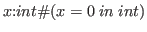
When we write
we are
really asserting the equality
This equality is a type. If it is true it is inhabited by.
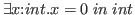
As another example of this interpretation, consider the goal.
This can be proved by introducing.
This is proved by introduction, and the inhabiting witness is.
Sets and Quotients
We
conclude the introduction of the type theory with
some remarks about two, more complex type constructors, the subtype
constructor and the quotient type constructor.
Informal reasoning about functions and types involves the
concept of subtypes.
A general way to specify subtypes uses a concept similar
to the set comprehension idea in set theory; that is,
![]() is the type of all
is the type of all ![]() of type
of type ![]() satisfying the
predicate
satisfying the
predicate ![]() .
For instance, the nonnegative integers
can be defined from the integers as
.
For instance, the nonnegative integers
can be defined from the integers as
![]() .
In Nuprl this is one of two ways to specify a subtype.
Another way is to use the type
.
In Nuprl this is one of two ways to specify a subtype.
Another way is to use the type
![]() .
Consider now two functions on the nonnegative integers
constructed in the following two ways.
.
Consider now two functions on the nonnegative integers
constructed in the following two ways.
The function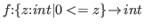
The difference between these notions of subset is more pronounced with a more involved example. Suppose that we consider the following two types defining integer functions having zeros.
It is easy to define a function

 .
(Notice that
.
(Notice that  .
There is no such function
.
There is no such function
One can think of the set constructor, ![]() , as serving
two purposes.
One is to provide a subtype concept; this purpose is
shared with
, as serving
two purposes.
One is to provide a subtype concept; this purpose is
shared with ![]() .
The other is to provide a mechanism for hiding information
to simplify computation.
.
The other is to provide a mechanism for hiding information
to simplify computation.
The quotient operator builds a new type from a given
base type, ![]() , and an equivalence relation,
, and an equivalence relation, ![]() , on
, on ![]() .
The syntax for the quotient is
.
The syntax for the quotient is ![]() .
In this type the equality relation is
.
In this type the equality relation is ![]() ,
so the quotient operator is a way of redefining equality
in a type.
,
so the quotient operator is a way of redefining equality
in a type.
In order to define a function
![]() one must
show that the operation respects
one must
show that the operation respects ![]() , that is,
, that is, ![]() implies
implies
 .
Although the details of showing
.
Although the details of showing ![]() is well-defined may
be tedious, we are guaranteed that concepts defined in
terms of
is well-defined may
be tedious, we are guaranteed that concepts defined in
terms of ![]() and the other operators of the theory respect
equality on
and the other operators of the theory respect
equality on ![]() .
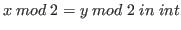
As an example of quotienting changing
the behavior of functions, consider defining the
integers modulo 2 as a quotient type.
.
As an example of quotienting changing
the behavior of functions, consider defining the
integers modulo 2 as a quotient type.
We can now show that successor is well-defined on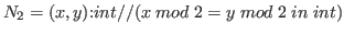
 then
then
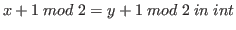 .
On the other hand, the maximum function is not well-defined
on
.
On the other hand, the maximum function is not well-defined
on  but
but 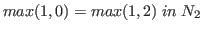 .
.
Semantics
This section is included for technical completeness; the beginning reader may wish to skip this section on a first reading. Here we shall consider only briefly the Nuprl semantics. The complete introduction appears in section 8.1. The semantics of Nuprl are given in terms of a system of computation and in terms of criteria for something being a type, for equality of types, for something being a member of a given type and for equality between members in a given type.
The basic objects of Nuprl are called terms. They are built using variables and operators, some of which bind variables in the usual sense. Each occurrence of a variable in a term is either free or bound. Examples of free and bound variables from other contexts are:
- Formulas of predicate logic, where the quantifiers (
 ,
,  )
are the binding operators. In
)
are the binding operators. In
 the two occurrences of
  are bound, and the occurrence
of
are bound, and the occurrence
of  is free.
- Definite integral notation. In
 the occurrence of is free, the first occurrence of is free, and
the other two occurrences are bound.
the occurrence of is free, the first occurrence of is free, and
the other two occurrences are bound.
- Function declarations in Pascal. In
function Q(y:integer):integer;
all occurrences of x and y are bound, but in the declaration of P x is bound and y is free.
function P(x:integer):integer; begin P:=x+y end ;
begin Q:=P(y) end ;
By a closed term we mean a term in which no variables are free. Central to the definitions of computation in the system is a procedure for evaluating closed terms. For some terms this procedure will not halt, and for some it will halt without specifying a result. When evaluation of a term does specify a result, this value will be a closed term called a canonical term. Each closed term is either canonical or noncanonical, and each canonical term has itself as value.
Certain closed terms are designated as types; we may write ``![]() type''
to mean that
type''
to mean that ![]() is a type.
Types always evaluate to canonical types.
Each type may have associated with it closed terms
which are called its members; we may write ``
is a type.
Types always evaluate to canonical types.
Each type may have associated with it closed terms
which are called its members; we may write ``![]() '' to mean
that
'' to mean
that ![]() is a member of
is a member of ![]() .
The members of a type are the (closed) terms that have as values the
canonical members of the type, so it is enough when specifiying the
membership of a type to specify its canonical members.
Also associated with each type is an equivalence relation on its
members called the equality in (or on) that type;
we write ``
.
The members of a type are the (closed) terms that have as values the
canonical members of the type, so it is enough when specifiying the
membership of a type to specify its canonical members.
Also associated with each type is an equivalence relation on its
members called the equality in (or on) that type;
we write ``![]() '' to mean that
'' to mean that ![]() and
and ![]() are members of
are members of ![]() which satisfy equality in
which satisfy equality in ![]() .
Members of a type are equal (in that type) if and only if their values
are equal (in that type).
.
Members of a type are equal (in that type) if and only if their values
are equal (in that type).
There is also an equivalence relation ![]() on types called type equality.
Two types are equal if and only if they evaluate to equal types.
Although equal types have the same membership and equality, in Nuprl
some unequal types also have the same membership and equality.
on types called type equality.
Two types are equal if and only if they evaluate to equal types.
Although equal types have the same membership and equality, in Nuprl
some unequal types also have the same membership and equality.
We shall want to have simultaneous substitution of terms, perhaps containing free variables, for free variables. The result of such a substitution is indicated thus:
where,
What follows describes inductively the type terms in Nuprl and their
canonical members. We use typewriter font to signify actual
Nuprl syntax.
The integers are the canonical members of the type int.
There are denumerably many atom constants (written as character strings
enclosed in quotes) which are the canonical members of the type atom.
The type void is empty. The type ![]() |
|![]() is a disjoint union
of types
is a disjoint union
of types ![]() and
and ![]() .
The terms inl(
.
The terms inl(![]() ) and inr(
) and inr(![]() ) are canonical members of
) are canonical members of
![]() |
|![]() so long as
so long as
![]() and
and ![]() . (The operator names inl and inr
are mnemonic for ``inject left'' and ``inject
right''.)
The canonical members of the cartesian
product type
. (The operator names inl and inr
are mnemonic for ``inject left'' and ``inject
right''.)
The canonical members of the cartesian
product type ![]() #
#![]() are the terms
<
are the terms
<![]() ,
,![]() > with
> with ![]() and
and ![]() .
If
.
If ![]() :
:![]() #
#![]() is a type then
is a type then ![]() is closed (all types are closed)
and only
is closed (all types are closed)
and only ![]() is free in
is free in ![]() .
The canonical members of a type
.
The canonical members of a type ![]() :
:![]() #
#![]() (``dependent product'')
are the terms <
(``dependent product'')
are the terms <![]() ,
,![]() > with
> with ![]() and
and ![]() .
Note that the type from which the
second component is selected may depend on the first component.
The occurrences of
.
Note that the type from which the
second component is selected may depend on the first component.
The occurrences of ![]() in
in ![]() become bound in
become bound in ![]() :
:![]() #
#![]() .
Any free variables of
.
Any free variables of ![]() , however, remain free in
, however, remain free in ![]() :
:![]() #
#![]() .
The
.
The ![]() in front of the colon is also bound, and indeed it is this position
in the term which determines which variable in
in front of the colon is also bound, and indeed it is this position
in the term which determines which variable in ![]() becomes bound.
The canonical members of the type
becomes bound.
The canonical members of the type ![]() list represent lists of members of
list represent lists of members of ![]() .
The empty list is represented by nil,
while a nonempty list with head
.
The empty list is represented by nil,
while a nonempty list with head ![]() and tail
and tail
![]() is
represented by
is
represented by ![]() .
.![]() ,
where
,
where ![]() evaluates to a member of the type
evaluates to a member of the type ![]() list.
list.
A term of the form ![]() (
(![]() ) is called an application
of
) is called an application
of ![]() to
to ![]() , and
, and ![]() is called its argument.
The members of type
is called its argument.
The members of type
![]() ->
->![]() are called functions, and each
canonical member is a lambda term,
are called functions, and each
canonical member is a lambda term, \![]() .
.![]() ,
whose application to any member of
,
whose application to any member of ![]() is a member of
is a member of ![]() .
The canonical members of a type
.
The canonical members of a type ![]() :
:![]() ->
->![]() ,
also called functions, are lambda terms
whose applications to any member
,
also called functions, are lambda terms
whose applications to any member ![]() of
of ![]() are members of
are members of ![]() .
In the term
.
In the term ![]() :
:![]() ->
->![]() the occurrences of
the occurrences of ![]() free in
free in ![]() become
bound, as does the
become
bound, as does the ![]() in front of the colon.
For these function types it is required that applications of a
member to equal members of
in front of the colon.
For these function types it is required that applications of a
member to equal members of ![]() be equal in the appropriate type.
be equal in the appropriate type.
The significance of some constructors derives from the representation
of propositions as types, where the
proposition represented by a type is true if and only if the type
is inhabited.
The term ![]() <
<![]() is a type if
is a type if ![]() and
and ![]() are
members of int, and it is inhabited
if and only if the value of
are
members of int, and it is inhabited
if and only if the value of ![]() is less than the value of
is less than the value of ![]() .
The term (
.
The term (![]() =
=![]() in
in ![]() ) is a type if
) is a type if ![]() and
and ![]() are members of
are members of ![]() ,
and it is inhabited if and only if
,
and it is inhabited if and only if ![]() .
The term (
.
The term (![]() =
=![]() in
in ![]() ) is also written (
) is also written (![]() in
in ![]() );
this term is a type and is inhabited if and only if
);
this term is a type and is inhabited if and only if ![]() .
.
Types of form {![]() |
|![]() } or {
} or {![]() :
:![]() |
|![]() } are called set types.
The set constructor provides a
device for specifying subtypes; for example, {x:int|0<x} has just
the positive integers as canonical members.
The type {
} are called set types.
The set constructor provides a
device for specifying subtypes; for example, {x:int|0<x} has just
the positive integers as canonical members.
The type {![]() |
|![]() } is inhabited if and only
if the types
} is inhabited if and only
if the types ![]() and
and ![]() are,
and if it is inhabited it has the same membership as
are,
and if it is inhabited it has the same membership as ![]() .
The members of a type {
.
The members of a type {![]() :
:![]() |
|![]() } are the
members
} are the
members ![]() of
of ![]() such that
such that ![]() is inhabited.
In {
is inhabited.
In {![]() :
:![]() |
|![]() }, the
}, the ![]() before the colon and the free
before the colon and the free ![]() 's of
's of ![]() become bound.
become bound.
Terms of the form ![]() //
//![]() and (
and (![]() ,
,![]() ):
):![]() //
//![]() are
called quotient types.
are
called quotient types.
![]() //
//![]() is a type only if
is a type only if ![]() is inhabited, in which
case
is inhabited, in which
case ![]() exactly when
exactly when ![]() and
and ![]() are members of
are members of ![]() .
Now consider (
.
Now consider (![]() ,
,![]() ):
):![]() //
//![]() .
This term denotes a type exactly when
.
This term denotes a type exactly when ![]() is a type,
is a type,
![]() is a type for
is a type for ![]() and
and ![]() in
in ![]() ,
and the relation
,
and the relation
![]() is an equivalence relation
over
is an equivalence relation
over ![]() in
in ![]() and
and ![]() .
If (
.
If (![]() ,
,![]() ):
):![]() //
//![]() is a type then its members are the members of
is a type then its members are the members of ![]() ;
the difference between this type and
;
the difference between this type and ![]() only arises in the
equality between elements. Briefly,
only arises in the
equality between elements. Briefly,
![]() if and
only if
if and
only if ![]() and
and ![]() are members of
are members of ![]() and
and ![]() is inhabited.
In (
is inhabited.
In (![]() ):
):![]() //
//![]() the
the ![]() and
and ![]() before the colon and the free
occurrences of
before the colon and the free
occurrences of ![]() and
and ![]() in
in ![]() become bound.
become bound.
Now consider equality on the types already discussed.
Members of int are equal
(in int) if and only if they have the same value. The same goes for type atom.
Canonical members of ![]() |
|![]() ,
, ![]() #
#![]() ,
,
![]() :
:![]() #
#![]() and
and ![]() list are
equal if and only if they have the same outermost operator and their
corresponding immediate subterms are equal (in the corresponding types).
Members of
list are
equal if and only if they have the same outermost operator and their
corresponding immediate subterms are equal (in the corresponding types).
Members of ![]() ->
->![]() or
or ![]() :
:![]() ->
->![]() are equal if and only if
their applications to any member
are equal if and only if
their applications to any member ![]() of
of ![]() are equal in
are equal in ![]() .
The types
.
The types ![]() <
<![]() and (
and (![]() =
=![]() in
in ![]() ) have
at most one canonical member, namely axiom, so equality is trivial.
Equality in {
) have
at most one canonical member, namely axiom, so equality is trivial.
Equality in {![]() :
:![]() |
|![]() } is just the
restriction of equality in
} is just the
restriction of equality in ![]() to {
to {![]() :
:![]() |
|![]() }, as is the equality
for {
}, as is the equality
for {![]() |
|![]() }.
}.
Now consider the so-called universes, U![]() (
(![]() positive).
The members of U
positive).
The members of U![]() are types. The universes are cumulative; that is,
if
are types. The universes are cumulative; that is,
if ![]() is less than
is less than ![]() then membership and equality in U
then membership and equality in U![]() are just
restrictions of membership and equality in U
are just
restrictions of membership and equality in U![]() . U
. U![]() is closed
under all the type-forming operations except formation
of U
is closed
under all the type-forming operations except formation
of U![]() for
for ![]() greater than or equal to
greater than or equal to ![]() .
Equality in U
.
Equality in U![]() is the restriction of type equality to members of U
is the restriction of type equality to members of U![]() .
.
With the type theory in hand we now turn to the Nuprl proof theory. The assertions that one tries to prove in the Nuprl system are called judgements. They have the form
where,
The criterion for a judgement being true
is to be found in the complete introduction to
the semantics.2.6Here we shall say a judgement
![]() is almost true if and only if
is almost true if and only if
![]()
if
![]()
That is, a sequent like the one above is almost true
exactly when substituting terms ![]() of type
of type ![]() (where
(where ![]() and
and ![]() may depend on
may depend on ![]() and
and ![]() for
for ![]() ) for the
corrseponding free variables in
) for the
corrseponding free variables in ![]() and
and ![]() results in a true
membership relation between
results in a true
membership relation between ![]() and
and ![]() .
.
It is not always necessary to declare a variable with every hypothesis in a hypothesis list. If a declared variable does not occur free in the conclusion, the extract term or any hypothesis, then the variable (and the colon following it) may be omitted.
In Nuprl it is not possible for the user to enter a complete
sequent directly; the extract term must be omitted.
In fact, a sequent is never displayed with its extract term.
The system has been designed so that upon completion of a proof,
the system automatically provides, or extracts, the extract term.
This is because in the standard mode of use
the user tries to prove that a certain type is inhabited without
regard to the identity of any member.
In this mode the user thinks of the type
(that is to be shown inhabited) as a proposition and assumes that it
is merely the truth of this proposition that the user wants to show.
When one does wish to show explicitly that ![]() or that
or that ![]() ,
one instead shows the type (
,
one instead shows the type (![]() =
= ![]() in
in ![]() )
or the type (
)
or the type (![]() in
in ![]() ) to be inhabited.2.7
) to be inhabited.2.7
The system can often extract a term from an incomplete proof when the extraction is independent of the extract terms of any unproven claims within the proof body. Of course, such unproven claims may still contribute to the truth of the proof's main claim. For example, it is possible to provide an incomplete proof of the untrue sequent » 1<1 [ext axiom], the extract term axiom being provided automatically.
Although the term extracted from a proof of a sequent is not displayed in the sequent, the term is accessible by other means through the name assigned to the proof in the user's library. In the current system proofs named in the user's library cannot be proofs of sequents with hypotheses.
Relationship to Set Theory
Type theory is similar to set theory in many ways, and
one who is unfamiliar with the subject may not see readily how to distinguish the two.
This section is intended to help.
A type is like a set in these respects: it has elements, there are
subtypes, and we can form products, unions and function spaces of types.
A type is unlike a set in many ways too; for instance, two sets are
considered equal exactly when they have the same elements,
whereas in Nuprl types
are equal only when they have the same structure.
For example, void and {x:int|x<x}
are both types with no members, but they are not equal.
The major differences between type theory and set theory emerge at a
global level.
That is, one cannot say much about the difference between the type int
of integers and the set Z of integers, but one can notice that in type theory
the concept of equality is given with each type, so we write
x=y in int and x=y in int#atom.
In set theory, on the other hand,
equality is an absolute concept defined once for all sets.
Moreover, set theory can be organized so that all objects of the theory
are sets, while
type theory requires certain primitive elements, such as individual
integers, pairs, and functions, which are
not types.
Another major global difference between the theories concerns the method
for building large types and large sets.
In set theory one can use the union and power set axioms to build progressively
larger sets.
In fact, given any indexed family of sets,
![]() ,
the union of these sets exists.
In type theory there are no union and power type operators.
Given a family of types S(x) indexed by A,
they can be put together into
a disjoint union, x:A#S(x), or into a product,
x:A->S(x), but there is no way to collect only the members of the S(x).
Large unstructured collections of types can be obtained only
from the universes, U1,U2,... .
,
the union of these sets exists.
In type theory there are no union and power type operators.
Given a family of types S(x) indexed by A,
they can be put together into
a disjoint union, x:A#S(x), or into a product,
x:A->S(x), but there is no way to collect only the members of the S(x).
Large unstructured collections of types can be obtained only
from the universes, U1,U2,... .
Another global difference between the two theories is that set theory typically
allows so-called impredicative set
formation in that a set can be defined in
terms of a collection which contains the set being defined.
For instance, the subgroup ![]() of a group
of a group ![]() generated by elements
generated by elements
![]() is often
defined to be the least among all subgroups of
is often
defined to be the least among all subgroups of ![]() containing the
containing the ![]() .
However, this definition requires quantifying over a collection containing
the set being defined.
The type theory presented here depends on no such impredicative concepts.
.
However, this definition requires quantifying over a collection containing
the set being defined.
The type theory presented here depends on no such impredicative concepts.
For set theories, such as Myhill's CST [Myhill 75], which do not employ impredicative concepts, Peter Aczel [Aczel 77,Aczel 78] has shown a method of defining such theories in a type theory similar to Nuprl.
Both type theory and set theory can play the role of a foundational theory. That is, the concepts used in these theories are fundamental. They can be taken as irreducible primitive ideas which are explained by a mixture of intuition and appeal to defining rules. The view of the world one gets from inside each theory is quite distinct. It seems to us that the view from type theory places more of the concepts of computer science in sharp focus and proper context than does the view from set theory.
Relationship to Programming Languages
In many ways the formalism presented here will resemble a functional programming
language with a rich type structure.
The functions of Nuprl are denoted by lambda expressions, written ![]() x.t,
and correspond to programs.
The function terms do not carry any type information, and they are evaluated
without regard to types.
This is the evaluation style of ML [Gordon, Milner, & Wadsworth 79], and it contrasts with a style in which
some type correctness is checked at runtime (as in PL/I).
The programs of Nuprl are rather simple in comparison to those of modern
production languages; there is no concurrency,
and there are few mechanisms to
optimize the evaluation (such as alternative parameter passing mechanisms,
pointer allocation schemes, etc.).
x.t,
and correspond to programs.
The function terms do not carry any type information, and they are evaluated
without regard to types.
This is the evaluation style of ML [Gordon, Milner, & Wadsworth 79], and it contrasts with a style in which
some type correctness is checked at runtime (as in PL/I).
The programs of Nuprl are rather simple in comparison to those of modern
production languages; there is no concurrency,
and there are few mechanisms to
optimize the evaluation (such as alternative parameter passing mechanisms,
pointer allocation schemes, etc.).
The type structure of Nuprl is much richer than that of any programming language; for example, no such language offers dependent products, sets, quotients and universes. On the other hand, many of the types and type constructors familiar from languages such as Algol 68, Simula 67, Pascal and Ada are available in some form in Nuprl. We discuss this briefly below.
A typical programming language will have among its primitive types the
integers, int, booleans, bool, characters, char, and
real numbers (of finite precision), real.
In Nuprl the type of integers, int, is provided; the booleans can be
defined using the set type as
{x:int | x=0 in int or x=1 in int},
the characters are given by atom, and various kinds of real numbers can be
defined (including infinite precision), although
no built-in finite precision
real type is as yet provided.
Many programming languages provide ways to build tuples of values.
In Algol the constructor is the structure; in Pascal and Ada it is the
record and has
the form
![]() for the product of types
for the product of types ![]() and
and ![]() .
In Nuprl such a product would be written A#B just as it would be in ML.
.
In Nuprl such a product would be written A#B just as it would be in ML.
In Pascal the variant record has the following form.
    RECORD
        CASE kind:(RECT,TRI,CIRC) of
            RECT:(w,h:real);
            CIRC:(r:real);
            TRI :(x,y,a:real)
    END
The elements of this type are either pairs, triples or quadruples, depending
on the first entry.
If the first entry is RECT then there are two more components,
both reals.
If the first entry is CIRC then there is only one other which is a real; if
it is TRI then there are three real components.
One might consider this type a discriminated union rather than a
variant record.
In any case, in Nuprl it is defined as an extension of the product operator which
we call a dependent product.
If real denotes the type of finite precision reals, and if the Pascal
type (RECT,CIRC,TRI) is represented by the type consisting of the three atoms
"RECT","CIRC" and "TRI", and if the function F is defined as
        F("RECT") = real#real
        F("CIRC") = real
        F("TRI")  = real#real#real
then the following type represents the variant record.
i:("RECT","CIRC","TRI")#F(i)
In Nuprl, as in Algol 68, it is possible to form directly the
disjoint union, written ![]() |
|![]() , of two types
, of two types ![]() and
and ![]() .
This constructor could also be used to define the variant record above as
real#real|(real|real#real#real).
.
This constructor could also be used to define the variant record above as
real#real|(real|real#real#real).
One of the major differences between Nuprl types and those of most programming
languages is that the type of functions from ![]() to
to ![]() , written
, written ![]() ->
->![]() ,
denotes exactly the total functions.
That is, for every input
,
denotes exactly the total functions.
That is, for every input ![]() of type
of type ![]() , a function in
, a function in
![]() ->
->![]() must produce a value in
must produce a value in ![]() .
In Algol the type of functions from A to B, say PROC(x:A)B, includes those
procedures which may not be well-defined on all inputs of A; that is,
they may
diverge on some inputs.
.
In Algol the type of functions from A to B, say PROC(x:A)B, includes those
procedures which may not be well-defined on all inputs of A; that is,
they may
diverge on some inputs.
In contrast to the usual state of affairs with programming languages the semantics of Nuprl ``programs'' is completely formal. There are rules to settle such issues as when two types of programs are equal, when one type is a subtype of another, when a ``program'' is correctly typed, etc. There are also rules for showing that ``programs'' meet their specifications. Thus Nuprl is related to programming languages in many of the ways that a programming logic or program verification system is.
Footnotes
- ... type.''2.1
- Actually
 reads as ``
 is a type
in universe .''
We discuss universes later.
is a type
in universe .''
We discuss universes later.
- ...2.2
- In full Nuprl the distinction between types and other objects is dropped.
- ... devices.2.3
- In Nuprl the goal
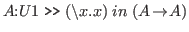 would
be expressed initially as
would
be expressed initially as
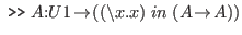 .
A rule of introduction would then create the context
.
A rule of introduction would then create the context  .
.
- ...2.4
- A better term to use here might be the token ``yes'',
which can be thought of as a summary of the proof.
The term
 suggests that the facts are somehow
basic or atomic, but in fact they may require
considerable work to prove.
suggests that the facts are somehow
basic or atomic, but in fact they may require
considerable work to prove.
- ....2.5
- In chapter 12 we introduce a concept of partial function
that will allow us to define
 such that
 using an unbounded search. The search is
guaranteed to terminate because of the information about
using an unbounded search. The search is
guaranteed to terminate because of the information about  .
.
- ... semantics.2.6
-
Section 8.1, page
![[*]](/icons/crossref.png) .
.
- ... inhabited.2.7
-
Recall that the term (
 =
=  in )
is a type whenever
in )
is a type whenever  and
and  and is inhabited just when
 .
As a special case the term ( in ), which is
shorthand for ( = in ), is a type and is inhabited
just when .
.
As a special case the term ( in ), which is
shorthand for ( = in ), is a type and is inhabited
just when .