PRL Home Introduction Math Library Publications Projects System

Seminar People The Book Lectures Other Groups

The Book

Implementing Mathematics with The Nuprl Proof Development System

The Terminal

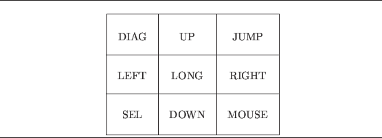
Nuprl is designed to run on a terminal with an ordinary keyboard with a control key, a keypad with nine keys arranged as in figure 3.2 and, optionally, a mouse. In the subsequent discussion we shall assume that these are available, and we shall assume that the mouse comes with three buttons called L, M and R (for left, middle and right, respectively) and is activated by clicking one of these buttons. However, one may simulate moving the mouse by using the keypad as follows. The arrow keys are used to move the cursor; if the arrow keys are used alone then the cursor moves in the direction of the arrow by either a single character or a single line. The cursor can be made to move in larger steps by pressing the key LONG #6586#>LONG} before the arrow key. The COMMAND #6587#>COMMAND} key is used for returning to the command window momentarily while in the middle of editing. For any particular terminal one may have to simulate the keypad and/or the mouse on the keyboard using control keys in combination with ordinary keys.

**Figure 3.2:** The Keypad
$\begin{figure}\hrule\vspace{12pt}\par \hbox to\hsize{ \hfil \hbox { \vbox {\of... ... }%end of inner hbox \hfil } %end of hbox. \par\vspace{2pt}\hrule \end{figure}$

#6588#>DIAG}#6589#> $\uparrow$ }#6590#>JUMP}#6591#> $\leftarrow$ }#6592#>LONG} #6593#> $\rightarrow$ }#6594#>SEL}#6595#> $\downarrow$ }#6596#>MOUSE}

The mouse is used for moving the cursor on the screen, for opening windows and for moving windows. An arrow on the screen called the mouse cursor responds directly to movements of the mouse. We shall also have occasion to refer to the cursor which responds to the keyboard and keypad commands as the cursor. To move the cursor, one places the mouse cursor at the desired position and clicks button R.

Windows

Users may control the placement and size of all windows. To alter a window, one places the cursor in it and invokes a menu by either clicking M on the mouse or simulating the mouse actions with the keypad in the following fashion. First, one enters mouse mode by pressing the MOUSE #6597#>MOUSE}key (see figure 3.2). Next, using the arrow keys and, optionally, the LONG #6598#>LONG} key, the user positions the mouse in the desired window and presses MOUSE again, thereby causing a menu of operations to appear. The option desired is selected by positioning the cursor next to the option in the displayed menu and pressing the MOUSE key; when a menu item is selected an asterisk appears on the left of the item. To leave mouse mode one uses the DIAG #6599#>DIAG}key. In subsequent discussion, the commands described are mouse commands rather than keypad commands. The translation to keypad commands is exactly as described in the discussion above.

The basic window manipulating commands available in the menu are size and move. The position of a window is determined by its upper left corner and the size by its lower right corner. To change position, for example, one selects the move option in the menu (by placing the cursor on it and clicking M) and then positions the cursor at the new location for the upper left corner and exits mouse mode by clicking M. Similarly, the size of the window can also be altered. Windows are closed by holding down the control key and pressing D. (The notation $\uparrow\!\!\mbox{D}$ is used to represent this key combination.) When a window is closed the cursor returns to the window it had been in when the new window was opened. Several other window management commands are available in mouse mode; these commands are typically needed when the user has several edit windows in use concurrently and needs to hide some of them temporarily. A complete discussion of these commands appears in chapter 7.

Commands and Status

Commands are used to enter objects in the library, to invoke editors, to check definitions, to save a session, to load back a saved session and to exit the system.^3.2Commands are entered into the command window by typing the text of the command at the prompt P> and ending with a carriage return. The system responds to commands by printing messages in the command window.

Starting Up

Nuprl is implemented in Lisp as a function; therefore, entering the Nuprl environment entails first invoking Lisp. Currently there are two implementations, one running on a Symbolics Lisp Machine and one written in Franz Lisp and running on Unix. One invokes the Nuprl environment using commands which load the system in the appropriate Lisp environment. The system comes up with a two-window display as in figure 3.3.

Figure 3.3: The Initial Display

,------------------------------,-----------------------,
| NuPRL Command/Status         | Library               |
|------------------------------|-----------------------|
|P>                            |                       |
|                              |                       |
|                              |                       |
'______________________________|_______________________'

P> is the top-level prompt from the command module. Depending on its mode, the window may display one of several prompts The modes and their corresponding prompts are:

P> Top-level Command Interpreter
I> Definition Facility
M> Metalanguage Interpreter
E> Evaluation Mechanism

In this chapter we discuss only the first two modes. The third mode is discussed in chapters 6 and 9, the fourth is discussed in chapters 5 and 7.

Finishing Up

After a session with Nuprl the results can be saved in the file system using the dump command as illustrated below. These files can then be reloaded with the load command. To end a session one uses the command exit.

Libraries

The library is the part of the system where objects of various kinds are stored. The system presents the user with a view of a portion of the library through the library window; the library window shows objects by name, kind (theorem, definition or ML), and status. For theorems, the statement of the theorem is also visible.

The scroll command alters the user's view of the library. The form of the command is scroll . This command moves the view down by the indicated number of objects; to move the view upward one uses the command scroll up.^3.3

Entry of Objects

One creates definitions and theorems in two stages. First, one creates a slot in the library where the new object is to be stored by issuing the create command followed by the name of the object, the kind of the object and a place for the name (top, bottom or before or after another name). The general form of the ``create'' command is create . An example of such a command follows.^3.4

        create t1 thm top

The result is the display of

 
        ? t1
        THM

as a new library entry. The system does not recognize this as an object but rather as a place where the object

will eventually reside. The mark ? is called a status mark. The status of an object can be any one of the following:

Incomplete: This applies only to theorems and means that the proof of the theorem is not completed. The status mark is #.
Good: This applies to any object and signifies that the object has been checked and found correct. In the case of a theorem, for example, it means that it has been proven. The status mark is $\ast$ .
Raw: The object has not yet been checked. The status mark is ?.
Bad: The object has been checked and been found incorrect. The status mark is -.

The second stage in creating an object involves invoking the proof and text editors on the library object created in the first stage described above. One does so by asking to view the object: view .^3.5Issuing view t1 results in a new window as shown in figure 3.4. If an object were present, it would appear in the window; at this stage, however, no object has been created, so one sees ? top. Since the object being edited is a theorem, the new window produced is a view of the proof editor, or refinement editor; if the object were a definition, then the system invokes the text editor. Definitions will be discussed at greater length in the next section. The refinement editor is a editor for tree-structured objects and is used for building proof trees. It is discussed in detail in chapter 4; at present it may be viewed as the place where theorems are displayed.

Figure 3.4: Appearance of the Screen after the Proof Editor Is Invoked

,------------------------------,
|EDIT THM t1                   |
|------------------------------|
|? top                         |                           
|<main proof goal>             |
|                              |
|                              |
|                              |
'------------------------------'---------------------------,
| NuPRL Command/Status         | Library                   |
|------------------------------|---------------------------|
|P>cr t1 thm top               |? t1                       |
|P>v t1                        |  THM                      |
|P>                            |                           |
|P>                            |                           |
'------------------------------'---------------------------'

To enter a theorem statement at this stage, one invokes the text editor (ted) by pressing the select key, SEL,#6600#>SEL} or by clicking the left key on the mouse with the mouse cursor in

main proof goal

. This opens a new window as shown in figure 3.5.^3.6These windows can of course be repositioned, resized or elided (moved off to the edge of the screen).

Figure 3.5: Appearance of the Screen after the Text Editor Is Invoked

,-------------------------------,---------------------------,
|EDIT THM t1                    |EDIT main goal of t1       |
|-------------------------------|---------------------------|
|? top                          |                           |
|<main proof goal>              |                           |
|                               |                           |
|                               '---------------------------'
|                               |
|                               |
'-------------------------------'---------------------------,
| NuPRL Command/Status          | Library                   |
|-------------------------------|---------------------------|
|P>cr t1 thm top                |? t1                       |
|P>v t1                         |  THM                      |
|P>                             |                           |
|P>                             |                           |
'-------------------------------'---------------------------'

One can now enter text into the text editor. As an example, suppose one were to type » 0=0 in int. This becomes the statement of the theorem t1 and makes the trivial assertion that

. The » symbol is our notation for the logical turnstile,^3.7 and the phrase in int appears because every statement of equality must be with respect to some type. One can now leave the text editor by pressing $\uparrow\!\!\mbox{D}$ ; the statement now appears in the proof-editing window. If one were trying to prove this theorem, one would at this stage start using the proof facilities to build the proof; this process is discussed in detail in chapter 4. For the present, one can simply exit from this window with $\uparrow\!\!\mbox{D}$ . The result is a new library entry for t1. The screen now looks like figure 3.6.

Figure 3.6: Appearance of Screen after Creating a Theorem

,-------------------------------,--------------------,
| NuPRL Command/Status          | Library            |
|-------------------------------|--------------------|
|P>cr t1 thm top                |# t1                |
|P>v t1                         |  THM >>0=0 in int  |
|P>                             |                    |
|                               |                    |
'-------------------------------'--------------------'

The status mark # indicates that this is an incomplete but syntactically correct object.

Saving Results

The library facility in Nuprl also allows one to save theorems, definitions and other objects produced in a session. For example, if it were desired to save the theorem t1 of the previous example in a file named library-name, one would issue the command

        dump t1 to library-name.

The theorem (together with its proof, if it has been proved) is stored in the file named in the dump command. If there is a library of several objects, say

        #t1
        THM ...

        #t2
        THM
        .
        .
        #tn
        THM

then the entire library can be saved by the command

        dump t1-tn to library-name

or by the command

        dump first-last to library-name.

Any segment of a library, say t5 to t9, can be saved by the command

        dump t5-t9 to library-name.

If one later wishes to retrieve a stored library, one issues the command

        load place from library-name,

where

refers to a place in the active system library and may be either top, bottom, before or after.

The Text Editor

Entering Text

The text editor is the basic tool which one uses to express anything in the Nuprl system. Even when using the proof editor to construct tree-structured proofs the text editor is constantly needed to communicate with the system; for instance, one uses it to tell Nuprl which proof rule to use. Entry of text in this editor is modeless; one types characters and deletes them as if using an ordinary keyboard. There are no special commands to ``save'' text or to ``write'' text. Text that exists in a window will be read and put in the library automatically when the window is closed.

Within the text editor one moves the cursor by using the mouse or the arrow keys on the keypad. Long moves of the cursor can be made by striking LONG once or twice before the arrow keys. One LONG#6601#>LONG} preceding a vertical arrow key moves the cursor up or down four lines; if used before a horizontal arrow key LONG moves the cursor left or right four positions. Two LONG's move the cursor to the end of the line if they precede a horizontal arrow key; if they precede a vertical arrow key they move the cursor up or down by a screenful. To move the cursor from one edit window to another the JUMP#6602#>JUMP} key is used.

Text is deleted using the delete key on the terminal or the kill key, KILL. The delete key removes the character to the left of the cursor, while the kill key removes the character at which the cursor is positioned. An entire region of text can be erased using the KILL key on a selected region. To select a region, the cursor is positioned at the beginning of the region and the SEL key is pressed or L is clicked. The cursor is then positioned at the end of the region and SEL is pressed again or L is clicked.^3.8 If the KILL key is used now the entire region is deleted and stored in a special buffer called the kill buffer. At most one region can be selected at a time; if three endpoints are selected only the last two are remembered. A kill operation causes the system to ``forget'' both the endpoints.

Copying Text

Text can be copied from one place to another in an edit window by selecting the region of text to be copied using the SEL key as before, placing the cursor where the selected text is to appear, and striking $\uparrow\!\!\mbox{C}$ . One may also copy text between edit windows by selecting text, jumping to the appropriate window using the JUMP key, placing the cursor at the appropriate spot and striking $\uparrow\!\!\mbox{C}$ .^3.9As with a kill operation, when a copy is performed the endpoints of the selected region are forgotten. If $\uparrow\!\!\mbox{C}$ is pressed while no region is selected then the contents of the kill buffer are copied at the cursor position. Using the copy operation in conjunction with the kill buffer does not destroy the contents of the kill buffer, so this is a convenient way to make multiple copies of a given piece of text.

Definitions

Nuprl provides a powerful and flexible definition facility which allows users to define their own notation. The general form of a definition follows:

$\begin{displaymath} text{\tt <}formal\: name\: {\tt :}\: description{\tt >}text\: {\tt ==}\: text. \end{displaymath}$

The left-hand side of a definition gives the form in which the definition is displayed when invoked; it gives the syntax of the extended notation. The right-hand side expresses the meaning of the new notation in terms of existing notation. The occurrences of <formal name:description> are parameters of the new notation. It is essential to use the angle brackets to enclose the parameters of a definition; otherwise, the symbol intended as a parameter will be used as a literal symbol every time the definition is instantiated. If the left angle bracket,

, is used as the less than symbol of number theory then it must be preceded by an escape character, $\backslash$ in the text editor, to prevent the system from interpreting the

as the start of a parameter to the definition. Most of the definitions shown in this chapter have the escape character removed in order to make the definitions more readable.

A definition is created in much the same way as a theorem is created. One opens a place in the library using the command create def . The object is then viewed by the command view , which in the case of a definition invokes the text editor rather than the proof editor. The form of the definition is now entered directly in the text editor. To illustrate this process suppose one wishes to define the logical connective ``and'' in terms of the type constructor #. A place in the library is first created using the create command; this command would include a name, say and, for the definition being created. The object and would then be viewed, and the text editor would thereby be invoked. In the text editor one would type

        <p:prop> & <q:prop> == ( (<p>) # (<q>) ).

Upon exit with $\uparrow\!\!\mbox{D}$ the system places the definition in the library.

Before a definition can be used it must be checked; this is done by issuing the command check . The system updates the status of the definition to either good, indicated by the status mark $\ast$ , or bad, indicated by the status mark -. Returning to our example, after and is checked, it extends the notation by introducing the new symbol &, which is defined in terms of the existing type constructor #.

To use a definition in creating another object, one types $\uparrow\!\!\mbox{I}$ in the text editor while editing the new object; the cursor will be put in the command window with the prompt being I>. The definition name is typed followed by a RETURN; the left-hand side of the definition appears where the cursor is positioned. Angle brackets containing the description will appear in the positions where a parameter is expected. In the example above, using the definition would result in the appearance of [<prop> & <prop> ]. The parameters, p and q in the example above, can now be entered by moving the cursor to the places indicated by angle brackets and typing the desired parameters. As the instantiations for the parameters are typed the angle brackets vanish. It is possible to use another definition while instantiating the parameters of a definition.

If one wishes to delete a definition then the kill command must be used. To delete an instance of a definition in another object, one positions the cursor at the beginning of the definition and hits the kill key. The easiest way to ensure that the cursor is correctly positioned is to use bracket mode. This is a display mode in which instantiated definitions are shown with brackets surrounding them and is normally the default mode. If the bracket display is not desired, bracket mode can be turned off by using $\uparrow\!\!\mbox{B}$ . This key serves as a toggle between the two display modes.

Syntactic Issues

The Nuprl system reads text from an edit window when that window is closed by typing $\uparrow\!\!\mbox{D}$ . The text is read by a parsing routine which will accept text that conforms to syntactic rules described in detail in section 8.1. These syntactic rules do not completely characterize the meaningful entities; thus the parser may accept text which cannot be viewed as a term. Essentially this means that the parser does not perform any type checking. Text which is accepted by the parser is called readable text. Text which is meaningful in the sense of the semantic account in chapter 2 is called readable and well-formed. Each well-formed piece of text is called a term. Note that our notion of well-formedness is semantic, unlike the traditional usage of the word ``well-formed''. The rest of this section contains a brief discussion of syntactic issues that are of immediate relevance.

Theorems

In Nuprl all theorems consist of goal statements, where a goal statement is similar to sequents used in natural deduction style inference systems. The form of a goal statement is » , where

is a hypothesis list and

is a formula in the Nuprl logic. The symbols » separate the hypotheses from the conclusion and thus correspond to the $\vdash$ symbol used in logic. Top-level goals must have empty hypothesis lists; this prevents the user from introducing inconsistent hypotheses. Theorems also cannot contain free variables; in the terminology of chapter 2, this means that all top-level goals must contain closed terms to the right of the » symbol.

Expressions Formed by Using Type Constructors

The basic components of the type theory employed by the Nuprl system are the atomic types int, atom and void. In addition to the atomic types, there is an integer-indexed family of predefined types called universes, $U_{1}, U_{2}, \ldots$ . Universes are types whose canonical elements are types. All the atomic types are members of

, and

is a member of $U_{i+1}$ . More complex types are built from the atomic types and the universes by using type constructors, operators which take types and build new types from them. The type constructors used in Nuprl are^3.10

`#`	product type constructor;
`->`	function type constructor;
`\|`	disjoint sum type constructor;
`x:A#B`	dependent product type constructor;
`x:A->B`	dependent function type constructor;
`A list`	list constructor;
`{x:A\|B}`	subset constructor;
`x,y:A//B`	quotient type constructor.

The meaning of these type constructors has been briefly discussed in chapter 2 and will be discussed in detail in chapter 8. The first three type constructors are binary, and all have equal precedence. They all associate to the right. We can also form types by using the forms ``in'' and `` = in ''. As explained in chapter 2, these are two of the basic judgement forms. The symbols in and = can be viewed as a type constructor for the purposes of the present discussion. Viewed in this way, in associates to the left. The symbol = binds more tightly than the symbol in. The type constructors in the list above also bind more tightly than does in. The binding and scope conventions are described in chapter 2.

Stating Theorems

The discussion so far has focused on the mechanics of using Nuprl. The rest of this chapter will concentrate on the conceptual issues that arise when one uses Nuprl to express formal mathematics. The discussion will continue to make reference to the mechanics of using Nuprl so that interested readers can take the opportunity to experiment with the system while familiarizing themselves with the logic of Nuprl. No attempt will be made to discuss proof techniques in this chapter; these will be covered in chapter 4.

All theorems in Nuprl have the form ``» '', where » separates assumptions from the goal. One can read »int in U1 as ``prove that type int is in from no assumptions.''^3.11In the next chapter we will see how various rules generate assumptions.

The most important aspect of the Nuprl system is the constructive nature of the type theory that underlies the system. A beginner should therefore be careful to make certain that the theorems being expressed are indeed constructively true. Even if a particular theorem is constructively true, the reader should remember that the proof will involve carrying out the actual constructions needed to exhibit the truth of the theorem. Thus several classically trivial theorems (or axioms) become relatively difficult. The benefit of the constructive viewpoint, of course, is that the resulting proofs become computationally significant. The heart of the constructive interpretation is contained in the propositions-as-types principle, which is discussed later in this section. It should be noted here that the constructive nature of the Nuprl type system in no way inhibits the possibility of modeling classical logic, and in fact we do so in the next section. The use of a constructive type theory for the Nuprl system is in sharp contrast to other systems for theory development, notably the LCF system.

Expressing Concepts in the Language of Types

The first example of formal mathematics that we shall consider is type theory itself. Since this is the ``primitive language'' of Nuprl it will not be necessary to write definitions; the basic constructors and atomic types are already available.

As we have already mentioned, the three atomic types are int, atom and void,^3.12and the types are classified into a cumulative hierarchy of universes, $U_{1}$ , $U_{2}$ , $\ldots$ .^3.13A type in universe $U_{i}$ is said to be at level . The atomic types all exist at level , i.e., in $U_{1}$ . We can express this for the type of integers with the statement int in U1. We now illustrate the mechanics of stating theorems one more time using this theorem as an example. Figure 3.7 shows actual snapshots of the screen as the theorem is produced. First, a position is created in the library using the command cr t1 thm bot. The proof editor is entered using v t1, and the text editor is entered by positioning the cursor on <main proof goal> and hitting SEL. We now type int in U1 in the text editor and then hit $\uparrow\!\!\mbox{D}$ .

Figure 3.7: Stating a Simple Theorem

   
,-----------------------------,----------------------------,
|EDIT THM t1                  |EDIT main goal of t1        |
|-----------------------------|----------------------------|
|? top                        |>> int in U1                |
|<main proof goal>            |                            |
|                             |                            |
|                             |                            |
|                             '----------------------------'
|                             |
'-----------------------------'----------------------------,
| NuPRL Command/Status        | Library  (first_session)   |
|-----------------------------|----------------------------|
|P>cr t1 thm bot              |? t1                        |
|P>v t1                       |  THM                       |
|                             |                            |
|                             |                            |
'-----------------------------'----------------------------'

Propositions as Types

The theorems we have seen so far have appeared rather ordinary, but their semantics suggests another kind of statement which is not. The interpretation we discuss below may seem problematic to the reader who is seeing constructive mathematics for the first time, so it may be useful for the new user to contrast the ideas below with the traditional, truth-functional view of the semantics of logic. In constructive logic a proposition is identified with the evidence we can give for it. Specifically, a proposition is a type consisting of formal objects called proofs.^3.14For example, the proofs corresponding to 0=0 in int and to int in U1 consist solely of the object axiom. It is important to note that although we think of statements of membership (e.g., 1 in int) or of equality (e.g., 0=0 in int) as being propositions, they are in fact types and they are combined with other types using type constructors. Later on we show how to define logical connectives in terms of type constructors so that we can combine these kinds of statements in the familiar fashion of sentential logic. As far as the Nuprl system is concerned, however, propositions are just types.

With this view of propositions, we lose some of the equivalences of classical logic. Thus, for example, if is a proposition and $\sim \! p$ represents its negation then and $\sim \sim \! p$ are no longer equivalent. As types they are different, although from a classical, truth-functional point of view they are the same.

Not only can we assert types which correspond to propositions by exhibiting (either explicitly or implicitly) members of the type, but it makes sense to assert any type. To do so means that the type is inhabited. To prove the assertion is to produce an object, either implicitly or explicitly.^3.15

Defining Logics

In this section we shall show how one can use the type theory described above to define various logics. The general pattern of presentation will be as follows:

A series of definitions is introduced so that one can work directly with familiar logical notation instead of the underlying type-theoretic notation.
Theorems are stated using the defined notation.

Constructive Logic

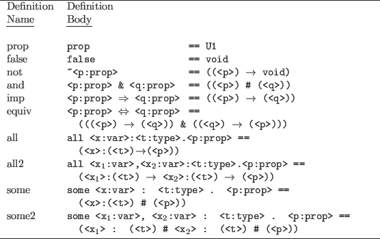
The first example of a logic that we express in type theory is constructive logic. This logic is very close in spirit to the constructive principles underlying type theory, so expressing constructive logic amounts to interpreting the type constructors of the Nuprl logic as logical connectives using the informal semantics of evidence that was employed in the discussion of propositions as types.

The definitions in figure 3.8 ^3.16 express the correspondence between logical connectives and type constructors.

We treat $A \: or \: B$ as $A\mid B$ , so we do not need an explicit definition for the usual logical ``or'' in terms of the type constructors. We could also include notations all3, some3, all4, etc., for higher numbers of variables of the same type, but in practice two or three suffice most of the time.

The rules for the logical operators defined in this way are exactly the rules for constructive logic; see for example [Dummet 77]. We will discuss this at length in chapter 4 when we study proofs and rules; however, one can see the intentions behind these definitions in terms of an informal semantics of evidence of the kind mentioned in chapter 1. Consider first the definition and; there is evidence for & precisely when there is a pair, $<\! a,b\! >$ , such that is evidence for and is evidence for . Thus treating & as # is semantically correct from this viewpoint.

Consider $A \; or \; B$ next. According to the constructive interpretation, $A \; or \; B$ is true when we have evidence for or for and when we can tell from the evidence which of or it supports. This is precisely the information that is available in the type $A\!\mid\! B$ . An element of the disjoint union is either or , where is in and is in and and are the canonical injections into the disjoint sum type.

Next consider $A\!\Rightarrow\! B$ . According to Brouwer [Brouwer 23], the founder of Intuitionism, an implication is true when there is a method of transforming any evidence for the antecedent, , into evidence for the consequent, . If and are represented by types, then the function space, $A \!\rightarrow\! B$ , consists of objects which are in fact evidence for $A\!\Rightarrow\! B$ . Thus our definition is semantically correct. The definition of the biconditional, $A\!\Leftrightarrow\! B$ , is correct given that the definition of implication is correct.

The constructive meaning of negation is delicate. To say is to say that there is no evidence for or that will never be proved. In a type-theoretic context one way to know this is to see that there are no members in . One might be tempted to translate as , but type equality means more than simply having the same members. To say is empty, we can say is equivalent to void, i.e., that $A\rightarrow Void$ # $Void\rightarrow A$ . However, $Void\rightarrow A$ is always inhabited, so the only new content is $A\rightarrow Void$ , which we take as our definition of .^3.17

**Figure 3.8:** Constructive Logic Connectives Expressed as Types
$\begin{figure}\hrule \begin{tt} \begin{tabular}{ll} {\rm Definition}& {\rm Defin... ...: (<t>) \char93 (<p>))\\ \end{tabular}\end{tt} \vspace{2pt}\hrule \end{figure}$

Now consider , which is read ``we can find an x of type such that is true.'' Intuitively there is evidence for an assertion of existence when we have a witness, in , and evidence, , that is true with substituted for free variable in . We write this substitution as . The dependent sum type # consists of pairs $<\! a,b\! >$ with exactly these properties, so the definition is correct.

A universal statement, , means constructively that given any element of we can find evidence for . This means that there is a procedure mapping elements of into . This is precisely what the dependent function space $x:A\rightarrow B$ provides, so this definition is also correct.

Finally, there should be no evidence for , so the empty type, , is the right definition for it.

These definitions can be applied to atomic propositional forms such as the types x = y in int or x < y to produce statements such as all x:int.some y:int. x<y, which we read as ``for all integers we can find some integer such that is less than ''. It is also possible to make more general statements, such as all A:U1.all x:A.x=x in A. This statement says that equality on every type is reflexive and involves quantifying over all types in $U_{1}$ ; without the hierarchy of universes it would not be possible to make such a statement predicatively.

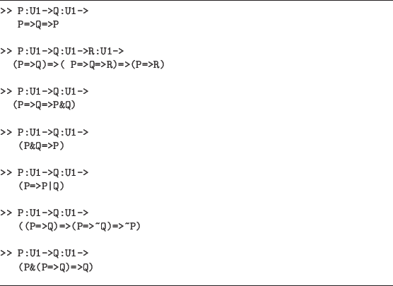
The logical operators can be used to state general results about constructive predicate logic. Give the identification of propositions and types, which we can make more conspicuous by the definition prop == U1, we can assert theorems about constructive propositional logic. Figure 3.9 gives a list of theorems that were expressed and proved in Nuprl.

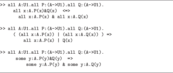
**Figure 3.9:** Some Theorems of Constructive Propositional Logic
$\begin{figure}\hrule \begin{verbatim}>> P:U1->Q:U1-> P=>Q=>P >> P:U1->Q... ... >> P:U1->Q:U1-> (P&(P=>Q)=>Q)\end{verbatim} \vspace{2pt}\hrule \end{figure}$

Statements in the predicate calculus are usually analyzed, following Frege [Frege 1879], as operators applied to propositional functions, where the term propositional function describes a function that maps objects to propositions. Given a type , the propositional functions (of one argument) on are of the type $A\rightarrow U_{1}$ . With this reading some basic facts from the predicate calculus are shown in figure 3.10.

**Figure 3.10:** Some Predicate Calculus Theorems
$\begin{figure}\hrule \begin{verbatim}>> all A:U1.all P:(A->U1).all Q:(A->U1).... ...=> some y:A.P(y) & some y:A.Q(y)\end{verbatim} \vspace{2pt}\hrule \end{figure}$

Classical Logic

It is possible to express classical logic in the Nuprl system by introducing appropriate definitions. More specifically, one can introduce a logical connective to correspond to the classical ``or'' by defining the new connective via the classical equivalence between ``or'' and a suitable combination of ``not'' and ``and''. Consider the additional logical operators defined in figure 3.11. The ``vel'' operator represents the classical connective ``or''.^3.18The classical notion of implication is usually called material implication and is defined in terms of vel just as shown in figure 3.11. Likewise, the classical idea of existence is far different from the constructive notion of existence in that we can prove something exists classically by merely showing that it is contradictory for it not to exist. This is precisely the meaning captured by the given definition.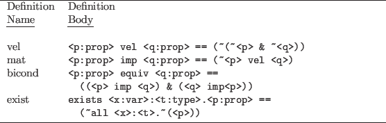

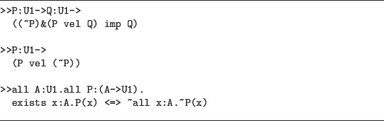
**Figure 3.11:** Definitions for Classical Logic
$\begin{figure}\hrule \begin{tt} \begin{tabular}{ll} {\rm Definition}& {\rm Defin... ...l <x>:<t>.\tilde (<p>))\\ \end{tabular}\end{tt} \vspace{2pt}\hrule \end{figure}$

Figure 3.12 shows some of the laws of classical logic in our notation.

From a formal point of view the situation is clear. We have defined logical operators that obey the laws of classical logic and are thus complete for the classical concept of logical truth in the first-order case. We have given an explanation of these laws in terms of type-theoretic concepts. While this is not the usual explanation in terms of Tarski's truth semantics, it is an adequate explanation for first-order logic.

**Figure 3.12:** Some Laws of Classical Logic
$\begin{figure}\hrule \begin{verbatim}>>P:U1->Q:U1-> ((~P)&(P vel Q) imp Q) ... ...exists x:A.P(x) <=> ~all x:A.~P(x)\end{verbatim} \vspace{2pt}\hrule \end{figure}$

Other Logical Operators

A number of other logical concepts can be expressed in Nuprl. For example, the conditional and is sometimes used when dealing with partial functions. This connective can be defined as <p:prop> cand <q:prop> == (x:<p> # <q>). This results in an and connective which forces the evaluation of its first argument before the second argument.

As another example, sometimes it is useful to simplify the structure of a type considered as a proposition by ``squashing'' all of the proofs into one object. This squash operator is defined as

        || <p:prop> || == {0 in int | <p> }.

Thus if <p> is true then || <p> || consists of a single object; all the different proofs have been identified. Note that this operator is built using the subset type constructor.

Elementary Number Theory

One of the atomic types available in Nuprl is the type integer, called int. The availability of integers as an atomic type allows one to express a great deal of elementary number theory without much effort. The type int comes equipped with an induction form so that one can inductively define functions from integers to integers. In this section we illustrate how some number-theoretic predicates and functions can be defined in Nuprl and how number-theoretic theorems are stated.

We begin this section with an example of a simple theorem which will be proved in chapter 4; we use this theorem to review how one enters theorems in the system. The theorem asserts that for every pair of integers one can find an integer whose value is 0 if the first of the original pair of integers is less than the second and whose value is 1 if the first of the original pair of integers is not less that the second. In this statement there are a pair of quantifiers; the first is universal and the second is existential. Accordingly we need the definitions for universal quantifiers and existential quantifiers from figure 3.8. To state the theorm in Nuprl, one would first create a name and place for the theorem using the commands discussed in section 3.2. Then the theorem would be viewed and finally the text editor would be invoked by clicking R on the mouse in <main proof goal>. Once in the text editor the first symbols typed would be »; after this the text of the theorem can be typed. At this stage the definition all2 is needed. We use it by first typing $\uparrow\!\!\mbox{I}$ ; this will put the cursor in the command window with the I> prompt. Now one types all2 followed by a carriage return. The definition will be instantiated in the text editor. The appearance of the definition template will be all <var>,<var>:<type>.<prop>. The variables x and y can now be entered as the first two parameters, and int can be entered as the third parameter. The body of this universally quantified statement is an existentially quantified statement. The last parameter, <prop>, in the definition is instantiated by invoking the definition for some. The first two arguments of this quantifier can be filled in as before. The body of the inner quantified statement is a conjunction of the two conditions appearing in the statement of the theorem and can be expressed using the built-in relation < between integers and the definitions for conjunction and negation. The final appearance of the theorem is as follows.

        >>all x,y:int. some z:int. 
            (x<y => z=0) & (~x<y => z= 1)

This is a theorem whose proof will embody some computational content; the existence proof will involve a procedure which computes

, given

and

The following definitions suggest what some standard number theory looks like in Nuprl. We first define the predicate divides using the (built-in) mod function.

        divides(<n>:int,<m>:int) == ( <m> mod <n> = 0 in int)

The next definition defines the predicate prime on integers.

        prime(<n:int>) ==
                 (1 < <n>) &   
                 all k:int. ( (0 < k) & 
                   (<n> mod k = 0  in int) ) =>
                     (k=1 in int) | (k=<n> in int)

Now these number-theoretic predicates can be used in conjunction with the logic definitions to state theorems in number theory in the following fashion.

        >> all n:int. prime(n) | ~prime(n)

        >> all n:int. some p:int. n<p & prime(p)

In stating number-theoretic propositions we come across our first examples of Nuprl theorems that have manifestly interesting computational content. The Nuprl system can extract the procedure from the proof. If we call the theorem t, then

        \n.(term_of(t)(n))

is a function which takes a natural number to a prime which is greater than it, where the function term_of is the system function that performs function extraction. Similarly the proof of the first theorem above will involve giving a decision procedure for primality.

Another interesting theorem one can state in Nuprl is the remainder theorem:

        >>all x:int. all y: int. some q:int. some r:int.
        	(y = (q*x + r) in int) & (0 <= r < x).

We assume that the term (0 <= r < x) has been defined to have its usual meaning via a definition.^3.19Once again a proof would give rise to an algorithm for finding the quotient and remainder resulting from dividing two integers, and the corresponding function would be extracted by the system. This illustrates, in a very simple setting, the use of Nuprl as a program synthesis tool.

Set Theory

The Subset Constructor

The expression of concepts from set theory in Nuprl is facilitated by the availability of the set type constructor as one of the primitive constructors of the underlying Nuprl logic. The notation for this constructor is {x:A|B}. Intuitively the set type constructor first forms a dependent sum of the two component types and then discards the second member of each pair in the dependent sum. The members of this type are those members

of the type

such that

is inhabited. Recalling the propositions-as-types principle, we may think of

as a propositional function and

as a proposition. The proposition

is true when the corresponding type is inhabited; thus the notation {x:A|B} defines the type whose members are members

that make the proposition

true. This is essentially what the classical set formation construct means.

The simplest statements about sets that one can make involve subsets of a specific type such as int. In Nuprl we may represent such sets as set types over int in the following fashion. Given a predicate on the integers, the set corresponding to is,

        {x:int | P(x)}.

This set type denotes those elements of int which satisfy

. Two important aspects of this type are that its members are elements of int and that the proof of

for an element

of int is not available in computations. For example, to prove that 9 belongs to

        {x:int | some y:int. ~(y=x in int) & x mod y=0 in int}

we must prove that some number, such as 3, satisfies the defining predicate, but we do not keep this factor as part of the membership condition. This means that from an assumption such as y in {x:int | P(x)} we do not have access to the proof of

. This aspect of the subset constructor comes out as a restriction on the way hypotheses can be used in the set-elimination rule.

Intervals

Subsets of the integers of the form $n, n+1, \ldots, n+p$ are especially useful. We call them intervals, and they are defined as follows. First we define the symbol <= to mean ``less than or equal to'' with the following definition:

        <x:int>\<=<y:int>==((<y><<x>)->void)}.

Now the concept of interval can be defined by

        {<n:int>,...,<m:int>}=={x:int| <n><=x # x<=<m>}.

Using intervals we can define the concept of an array a of type A as

        a:{1,...,n}->A.

A very important concept in set theory is the concept of equal cardinality. We shall use the term equipollent to signify the type-theoretic analogue of equal cardinality. As in classical set theory, two types are equipollent if there are a pair of invertible functions between them. This is captured by the following definition.

        <A:type> is equipollent with <B:type>==
        (some ab:<A>-><B>.some ba:<B>-><A>.all x:<A>.all y:<B>.
        ba(ab(x))=x in <A> &  ab(ba(y))=y in <B>)

In the constructive account, however, we must exhibit the two functions that establish equipollence, so it is not permissible to use the Schroeder-Bernstein theorem, for example, to establish equipollence. Thus equipollence is not identical to the classical notion of equal cardinality.

The following three Nuprl theorems express basic facts about equipollence.

        >>all A:U1.  A is equipollent with A          

        >>all A:U1.all B:U1. A is equipollent with B =>
          B is equipollent with A                    

        >>all A:U1.all B:U1.all C:U1.  
              A is equipollent with B &
                B is equipollent with C  =>
                   A is equipollent with C

Using the notions of intervals and equipollence we can define the concept of a finite type. We say that a type is finite if and only if it is equipollent with some interval.

        <A:type> is finite== some n:int.{1,...,n} is   
        equipollent with <A>

We say that

is the cardinality of A.

A nontrivial statement that can be made with the definitions introduced in this section is the pigeonhole principle. The following Nuprl theorem expresses the principle.

        >>all n:int.all m:int. all f:{1,...,m}->{1,...,n}.
              0<n<m => some i,j:int.i<j & f(i)=f(j) in int

The proof of such a proposition in Nuprl will include a procedure which, given a function

from the interval $\{ 1,\ldots,m \}$ to the interval $\{ 1,\ldots,n \}$ with

, produces the values

and

for which

. The constructive proof is considerably harder than the (trivial) proof of the classically interpreted pigeon-hole principle, but the information contained in the constructive proof is correspondingly much greater.

Algebra

In this section we examine a fragment of group theory and discuss how the definition of algebraic structures can be cast in the Nuprl logic. Defining an algebraic structure involves identifying certain distinguished functions (the operators) and constants and stating the properties of the functions and constants. The properties one wishes to state are usually equational and thus correspond to Nuprl terms. Expressing inequations is slightly more tedious but does not present any fundamental difficulty.

We begin by discussing how some typical phrases that one might see in an algebra text are expressed in Nuprl. Suppose one wishes to make a statement of the following general form: `` ''. In the first equation of such a statement the variable serves as an abbreviation for the right-hand side of the second equation. The entire statement thus expresses whatever the first equation expresses with appropriately instantiated. A natural way to express instantiation involves the application of a lambda term to another term. Thus we are led to the following Nuprl definition:^3.20

        <t:term> where <x:var>=<tt:term> == (\ <x>.<t>)(<tt>).

In algebra it is customary to write binary operators in infix form. In the Nuprl notation operators are just functions (lambda terms) expressed in curried form. The following definition thus allows one to use traditional algebraic syntax in discussing operators:

        <x:arg> <op:operation> <y:arg> == <op>(<x>)(<y>).

An important property of operators that one might wish to state is the property of associativity. Associativity is an equationally stated property; accordingly in Nuprl it is necessary to state associativity with respect to a particular type. One can use the definition for the universal quantifier in writing the definition of associativity to obtain the following definition.

        <op:A->A->A> associative over <A:type>== 
        All x,y,z:<A>. 
          x <op> (y <op> z) = (x <op> y) <op> z  in <A>

During an instantiation of the last definition the template displayed in the library window will look like the following:

        <A->A->A> associative over <A:type>.

With the definitions above, one can state the definition of a group. A group is just a type; accordingly the definition of a group will be a type expression in which the various components of the definition are pieced together. The complete definition is as follows:

        Group ==
          A:U1
        # o:(A->A->A)
        # e:A
        # All x:A.  x o e = e o x = x  in A 
        # All x:A. Some y:A.  x o y = y o x = e  in A 
        # o associative over A

In the definition above, o is the group composition operator, e is the group identity, and the last three lines express the standard properties of a group. There are a number of different ways in which the definition can be used in stating theorems. One could, for example, state the type Group as a top-level goal. This would then assert that there exist groups. One could make a statement of the form B in Group; this would assert that B is a group. A proof of such a statement would of course be constructive and would involve displaying a procedure for computing inverses in B. A third way of using the definition of a group would be to state properties true of all groups with statements of the form

        All G:Group. ... .

To be able to state interesting theorems about group theory it is necessary to be able to pull apart the constituents of a group. This is done using the spread operator, the elimination form of the product constructor. The following two definitions provide mnemonic access functions.

        fst(<x:term>) == spread(<x>;u,v.u)

        snd(<x:term>) == spread(<x>;u,v.v)

Now we can define notation that accesses the definition of a group and produces the underlying carrier set and operations. For example, the following definition defines the carrier set of a group.

        |<G:Group>| == fst(<G>)

We can access the composition operator and the identity of the group by using the following definitions.

        op_of <G:Group> == fst(snd(<G>)) 
	
        id_of <G:Group> == fst(snd(snd(<G>)))

We conclude this section by stating a typical elementary theorem of group theory, namely that every equation of the form $a\circ x = b$ can be uniquely solved for

. In Nuprl this theorem would read

        >> All G:Group. All a,b:|G|. 
           Some x:|G|. 
             (a o x = b in |G| 
              & All c:|G|. a o c = b in |G| => c = x in |G|
              where o=op_of G )

In the statement above, the fourth line states the uniqueness of the solution.

Footnotes

... system.^3.2: Other commands needed for proving theorems, evaluating terms, etc., will be discussed in later chapters.
... CLASS="MATH">.^3.3: The keyword scroll can be abbreviated by scr.
...^3.4: The keyword create can be abbreviated by cr.
... CLASS="MATH">.^3.5: The keyword view can be abbreviated by v.
...afterthm.^3.6: The new window is dependent on the first window, so the first window cannot be deleted until the text editor window is closed. The first window can, however, be moved off the screen by using the window-moving commands. Thus windows can be temporarily hidden.
...^3.7: The notation » is used instead of the more usual turnstile $\vdash$ since the former is available on most terminals.
... clicked.^3.8: Actually one can select the endpoints in either order.
... CLASS="MATH"> $\uparrow\!\!\mbox{C}$ .^3.9: One must not be in mouse mode while doing this.
... are ^3.10: Other type constructors are being actively investigated. Some of these will be discussed in chapter 12.
...^3.11: Although » must be present in every theorem, the system does not generate it because we want to allow the possibility of stating theorems with hypotheses, theorems such as x in int » x+1 in int.
...void,^3.12: This is not a mathematical fact but a fact about Nuprl, so we would not expect to be able to prove in Nuprl a theorem of the form ``if A is an atomic type, then A = atom or A = void''.
....^3.13: The notation $U_{i}$ is used in general discussion about the logic of Nuprl, whereas the notation Ui is used in discussing text used by Nuprl.
....^3.14: The proofs we are referring to in this discussion are not formal Nuprl proofs but abstract proofs.
...^3.15: Every object can be constructed in two ways, either explicitly as in the example above or implicitly. Every proof builds an object implicitly. We will see in chapter 4 how to prove implicitly that the integers are an object in .
...cldefs ^3.16: It is important to enclose the right side of the definition in parentheses to guarantee proper precedence and scope. Also, it is important not to include a carriage return in the definition. The carriage return will sometimes be read as a bad character when parsing the right side, but it will not be visible on the screen.
....^3.17: We will see other definitions later which will take account of the structure of .
...^3.18: The usual sign for classical or is $\lor$ , which abbreviates the Latin , meaning or. We have chosen not to use the word ``or'' at all among the logical operators because it has so many meanings in natural language.
... definition.^3.19: If the symbol is being used in a definition to mean ``less than'' then it must be preceded by a backslash; otherwise, the system will try to interpret it as the start of a new parameter.
... definition:^3.20: The space after the `` $\backslash$ '' in the definition is to prevent the parser from thinking that the following is being quoted.